Mechanical Calculators and Automata: From Ancient Counting Devices and Geared Mechanisms to Programmable Machines and the Foundations of Artificial Intelligence

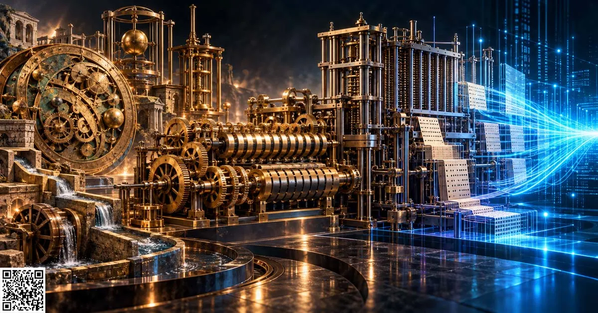
Long before the invention of electronic computers, microprocessors, neural networks, and modern artificial intelligence, human civilizations developed physical instruments capable of representing numerical quantities, simplifying mathematical operations, regulating mechanical movement, and executing predetermined sequences of actions.

These inventions established important foundations for the eventual mechanization of computation.

Counting boards and abacuses allowed numerical operations to be represented through the positions of physical objects. Astronomical instruments translated mathematical relationships into geometric and mechanical configurations. Water-driven automata and mechanical clocks demonstrated how energy, timing, and control mechanisms could coordinate sequences of actions without continuous human manipulation.

During the seventeenth century, inventors developed increasingly sophisticated mechanical calculators capable of performing arithmetic through gears, digit wheels, carry mechanisms, and other precision components. During the eighteenth and nineteenth centuries, programmable automata, punched-card mechanisms, and automatic calculating engines demonstrated progressively richer relationships between stored instructions, mechanical execution, and information processing.

The history of these devices is essential for understanding several concepts that later became fundamental to computing and artificial intelligence:

Numerical representation: Encoding quantities through physical states.

Mechanical computation: Performing mathematical operations through controlled physical transformations.

Automation: Executing actions through a mechanism without continuous manual intervention.

State: Representing the current configuration of a device.

Control: Determining how a mechanism responds to inputs or internal conditions.

Feedback: Allowing measured conditions to influence subsequent physical behaviour.

Programmability: Changing a device’s operations through a configurable sequence or representation of instructions.

General-purpose computation: Performing a broad range of computational procedures rather than one permanently fixed task.

However, these concepts must be distinguished carefully.

An abacus is a powerful calculation aid, but its ordinary operation depends on a human manipulating the beads. A mechanical clock can execute precisely timed actions without possessing intelligence. A programmable automaton can produce sophisticated movement while lacking the ability to learn from experience. A nineteenth-century mechanical calculating engine can implement mathematical procedures without reasoning about their meaning.

Similarly, the existence of ancient or medieval mechanisms does not establish the existence of modern artificial intelligence in those periods.

Modern AI emerged through additional developments in formal logic, probability, mathematical computation, electronic engineering, algorithms, statistics, and machine learning.

The relationship between historical mechanical devices and contemporary AI is therefore one of important intellectual and engineering foundations, not direct technological equivalence.

This article investigates the historical development, mathematical principles, physical mechanisms, architectural innovations, and limitations of mechanical calculators and automata. It examines how machines gradually acquired the ability to represent numbers, manipulate states, perform controlled operations, and execute increasingly complex procedures.

It also explains why these developments were indispensable to the broader history of computation while remaining distinct from the adaptive and inferential capabilities associated with modern artificial intelligence.

---

1. DEEP DEFINITION

1.1. What Is a Mechanical Calculator?

A mechanical calculator is a physical device that performs or assists numerical computation through the movement, configuration, or interaction of mechanical components.

Depending on its design, these components may include:

• Beads or movable counters.
• Numbered wheels.
• Gears.
• Ratchets.
• Levers.
• Shafts.
• Cams.
• Stepped drums.
• Carry mechanisms.
• Rotating cylinders.
• Sliding scales.
• Mechanical registers.
• Printing mechanisms.

Mechanical calculators differ in their degree of automation.

Some require a human operator to perform the essential computational transformations.

Others internally coordinate arithmetic operations after the operator supplies an input and initiates a mechanism.

A counting board, for example, provides a structured physical representation of numerical values.

A Pascaline performs arithmetic through mechanically linked digit wheels.

A stepped-reckoner design extends mechanical arithmetic through mechanisms capable of supporting multiplication and division.

A difference engine automates a specialized numerical procedure through repeated addition.

These devices belong to different technical categories despite their common connection to calculation.

The Computer History Museum documents the development of calculating instruments from early manual devices to sophisticated mechanical calculators and later electronic systems [1][6].

1.2. What Is an Automaton?

An automaton is a constructed mechanism that performs actions through an organized arrangement of components, usually after being activated or supplied with energy.

The actions may be repetitive, sequential, conditional, or otherwise determined by the mechanism’s design.

Historical automata have included:

• Moving mechanical figures.
• Automated fountains.
• Hydraulic clocks.
• Mechanical musicians.
• Animated theatrical devices.
• Moving animal representations.
• Self-operating display mechanisms.
• Mechanical writing machines.
• Programmed weaving mechanisms.
• Automated measuring instruments.

An automaton may perform visible actions without calculating numerical results.

Conversely, a mechanical calculator may perform arithmetic without producing lifelike motion.

Some devices combine both functions.

A water clock with moving figures, for example, may measure the passage of time while activating an animated display.

The defining property of an automaton is not necessarily intelligence.

It is the production of mechanically organized behaviour with some degree of automatic execution.

1.3. Mechanical Calculation Versus Automation

Mechanical calculation and automation address different engineering objectives.

Mechanical calculation concerns the physical implementation of mathematical operations.

Automation concerns the execution of operations through a mechanism rather than continuous direct human control.

A machine can automate calculation.

It can also automate a nonnumerical activity.

For example, an automated fountain may regulate the movement of water without performing arithmetic in the conventional sense.

A mechanical calculator may compute a result while requiring an operator to turn a handle.

The two concepts overlap when a mechanism both executes automatically and transforms numerical information.

Dimension	Mechanical calculator	Mechanical automaton
Primary function	Numerical computation	Coordinated physical behaviour
Input	Numbers or physical quantities	Trigger, energy, time, or environmental condition
Internal representation	Digits, scales, gear positions	Mechanical states and control configurations
Typical output	Numerical result	Motion, sound, display, or physical action
Human involvement	Varies by design	Varies by design
Learning requirement	None	None
Example	Pascaline	Hydraulic theatrical figure
Shared foundation	Physical state, controlled transformation, and mechanical execution	Physical state, controlled transformation, and mechanical execution

This comparison explains why the histories of calculators and automata intersect without being identical.

1.4. Mechanical Calculation Versus Computation

The word computation has a broader meaning than arithmetic.

Arithmetic operations include addition, subtraction, multiplication, and division.

Computation may also involve symbolic manipulation, comparison, logical operations, iteration, conditional processing, and transformations of structured information.

A mechanical calculator may implement a restricted collection of arithmetic functions.

A programmable computing machine can, in principle, perform broader classes of procedures.

The distinction is particularly important when comparing Charles Babbage’s Difference Engine with his Analytical Engine.

The Difference Engine was designed to evaluate mathematical tables through a specialized method.

The Analytical Engine introduced a design for a much more general programmable calculating machine.

The Computer History Museum identifies this as a crucial transition from automated arithmetic to programmable computation [14].

However, programmability alone does not necessarily establish computational universality.

The actual instruction set, memory capacity, control mechanisms, and computational model must be considered.

1.5. Positional Number Representation

Mechanical computation depends fundamentally on methods for representing numerical values.

In a positional numeral system with base b, a nonnegative integer N can be expressed as:

N = Σᵢ₌₀ᵐ dᵢbⁱ

Where:

• b is the numerical base.
• dᵢ is the digit at position i.
• 0 ≤ dᵢ < b.
• m is the highest represented position.

For decimal notation:

b = 10

Consider:

N = 472

Its positional representation is:

472 = 4 × 10² + 7 × 10¹ + 2 × 10⁰

Therefore:

472 = 400 + 70 + 2

Mechanical calculators commonly represented these positional values through separate digit wheels or registers.

Each wheel corresponded to a particular power of ten.

The physical position of the wheel encoded the associated digit.

This relationship between symbolic numerical representation and physical state was central to the development of mechanical arithmetic.

1.6. Arithmetic as a Physical State Transformation

A mechanical calculator can be modeled retrospectively as a state-transition system.

Let:

S = (d₀, d₁, …, dₘ)

represent the current numerical register.

An input operation u changes the register according to:

Sₜ₊₁ = F(Sₜ, uₜ)

Where:

• Sₜ is the current machine state.
• uₜ represents an operator input or mechanical instruction.
• F is the physical transformation implemented by the mechanism.

For example:

Current state: 472

Operation: Add 38

New state: 510

The mechanism must perform the corresponding digit transformations and carry operations.

This formulation uses modern mathematical notation.

It does not imply that historical calculator inventors described their mechanisms in the language of contemporary state-transition theory.

Its purpose is to clarify the fundamental computational structure of their machines.

1.7. Exact and Approximate Mechanical Calculation

Mechanical calculating instruments can be divided into important categories according to how they represent quantities.

Discrete numerical mechanisms

These represent numbers through distinguishable states, such as digit-wheel positions or counting beads.

Under correct operation and sufficient capacity, they can perform exact integer arithmetic.

Continuous or analog mechanisms

These represent quantities through continuously varying physical properties, such as distance, rotation, or displacement.

Their precision depends on mechanical tolerances, calibration, observation, and physical measurement.

A slide rule, for example, performs approximate numerical operations through logarithmic scales.

A digit-wheel calculator performs arithmetic through discrete positional states.

Both are useful, but their precision characteristics differ.

A continuous mechanical device is not automatically more advanced than a discrete calculator.

The appropriate architecture depends on the required mathematical operations and accuracy.

1.8. Counting Boards and the Abacus

Counting boards and abacuses are among the most enduring calculation aids in human history.

They use physical counters or beads to represent numerical quantities through position.

Different forms developed across multiple civilizations.

Examples include:

Counting boards: Surfaces divided into numerical positions where counters are placed or moved.

Suanpan: A traditional Chinese abacus.

Soroban: A Japanese abacus.

Schoty: A Russian abacus.

Table abacus: A counting surface using movable markers or jetons.

The Computer History Museum documents the historical diversity of these instruments and their continuing importance in practical calculation [1].

The abacus demonstrates a fundamental principle of information processing:

Numerical information can be represented and transformed through controlled changes in physical configuration.

However, the ordinary abacus is not an autonomous computing machine.

The operator supplies the computational procedure by deciding how and when to move the counters.

1.9. Ancient Astronomical Calculation

Astronomical prediction created strong incentives for systematic numerical computation.

Ancient societies needed methods for interpreting celestial cycles, maintaining calendars, and predicting recurring astronomical events.

The relevant mathematical tasks could involve:

• Periodic motion.
• Angular relationships.
• Calendar cycles.
• Lunar phases.
• Eclipse cycles.
• Solar and lunar positions.
• Astronomical tables.

Some calculations were performed manually.

Others were supported by instruments representing geometric or cyclic relationships.

The Antikythera mechanism provides particularly important surviving evidence of the mechanical implementation of complex astronomical calculations in antiquity.

Its historical significance rests on documented gear mechanisms and inscriptions rather than mythological accounts.

1.10. The Antikythera Mechanism

The Antikythera mechanism is an ancient Greek geared astronomical calculator recovered from a shipwreck near the island of Antikythera.

It was discovered in the wreck in 1901.

Research generally places its manufacture around the late second century BCE, although questions concerning precise dating and original configuration remain subjects of scholarly investigation.

The surviving object consists of corroded fragments containing intricate bronze gearwork and inscriptions.

Its mechanisms were designed to represent and calculate relationships among astronomical cycles.

In a major 2006 study, Freeth and colleagues used high-resolution X-ray tomography and surface-imaging methods to investigate the surviving fragments [2].

Their work established important details concerning the device’s gearing, astronomical functions, lunar motion, and eclipse-related calculations.

The mechanism is widely described as an early analog astronomical computer.

However, it should not be confused with a general-purpose programmable digital computer.

Its physical architecture implemented specialized astronomical relationships.

1.11. Astronomical Cycles in the Antikythera Mechanism

The Antikythera mechanism incorporated knowledge of recurring astronomical cycles.

Two particularly important cycles are:

Metonic cycle

Approximately:

19 solar years ≈ 235 synodic months

This relationship supports coordination between solar years and lunar months.

Saros cycle

Approximately:

223 synodic months

This cycle is associated with the recurrence of similar eclipse configurations.

The mechanism used gear arrangements and dials to represent relevant cycles.

Its calculations were based on mathematical astronomical relationships understood within the ancient world.

However, modern reconstructions must distinguish what surviving components directly establish from what is inferred.

Freeth and colleagues proposed an extensive reconstruction of the device’s front astronomical display in 2021 [3].

Because much of the original mechanism is missing, some aspects of its planetary display remain reconstruction-dependent rather than directly observable.

1.12. Mechanical Ratios and Astronomical Prediction

Gears can transform rotational motion according to numerical ratios.

Consider two externally meshing gears.

Let:

• N₁ be the number of teeth on the driving gear.
• N₂ be the number of teeth on the driven gear.
• ω₁ be the driving gear’s angular velocity.
• ω₂ be the driven gear’s angular velocity.

For ideal external gearing:

ω₂ = −(N₁/N₂)ω₁

The negative sign indicates opposite rotation directions.

If a gear with 20 teeth drives a gear with 60 teeth:

ω₂ = −(20/60)ω₁

Therefore:

ω₂ = −ω₁/3

The driven gear rotates at one-third the magnitude of the driving gear’s angular velocity.

By combining gear ratios, a mechanism can encode relationships among cycles.

The Antikythera mechanism demonstrates the sophisticated use of this principle for astronomical representation.

Its exact internal functions must nevertheless be interpreted through the surviving evidence and scholarly reconstructions.

1.13. Hero of Alexandria and Mechanical Automata

Hero of Alexandria was an influential ancient technical writer associated with mechanics, mathematics, pneumatics, and automated devices.

His treatise on automata describes mechanical theatrical devices capable of producing coordinated performances.

These descriptions are important because they concern identifiable mechanisms rather than purely supernatural animation.

The University of Glasgow’s research project on Hero’s theatrical automata combines textual interpretation, engineering investigation, and experimental reconstruction [4].

The project distinguishes mobile and stationary automata described in the surviving tradition.

Their functions involved coordinated mechanical operations designed to produce theatrical effects.

The technical significance lies in the integration of movement, sequencing, energy, and performance.

However, the devices should not be described as learning robots or artificial general intelligence.

Their capabilities were determined by mechanical arrangements and the conditions under which those arrangements operated.

1.14. The Banū Mūsā and Hydraulic Engineering

The Banū Mūsā brothers—Muḥammad, Aḥmad, and al-Ḥasan ibn Mūsā ibn Shākir—were associated with important scientific and engineering work in the ninth-century Islamic world.

Their Kitāb al-Ḥiyal, usually translated as The Book of Ingenious Devices, describes mechanisms involving fluids, valves, containers, and other physical arrangements.

Donald R. Hill’s annotated English translation provides an important scholarly source for the work [5].

The devices illustrate the use of mechanical design to produce controlled physical effects.

Some mechanisms involve fluid pressure and flow regulation.

Others create sequences of behaviour through changes in physical conditions.

The historical significance includes increasingly sophisticated treatment of:

• Hydraulic behaviour.
• Mechanical regulation.
• Fluid pressure.
• Valve arrangements.
• Triggered movement.
• Controlled dispensing.
• Automated physical sequences.

These mechanisms provide important precedents for automation and control engineering.

However, their documented operation should not be interpreted as evidence of modern data-driven learning.

1.15. Al-Jazarī and Complex Automated Devices

Al-Jazarī, an engineer associated with the Artuqid court, completed an influential treatise on ingenious mechanical devices in the early thirteenth century.

The work describes approximately fifty devices organized into categories.

These include clocks, fountains, vessels, and mechanisms capable of producing coordinated movement.

The Smithsonian Institution preserves illustrated manuscript material associated with this technical tradition [6].

One documented example describes a clock involving figures, moving components, and mechanical signals.

The historical text and illustrations demonstrate the integration of technical knowledge with visual performance.

However, the surviving illustrated manuscripts may date from periods later than al-Jazarī himself.

A manuscript produced in 1315, for example, should not be identified as an original document physically created in 1206.

The distinction between original authorship, later manuscript copying, and modern reconstruction is essential to accurate historical interpretation.

1.16. Napier’s Bones

John Napier’s calculation rods, commonly called Napier’s bones, were described in his Rabdologiae in 1617.

They simplified multiplication and division through arrangements of numerical tables on physical rods.

The method transformed some multiplication tasks into operations involving the selection and addition of displayed partial products.

The Computer History Museum notes that the underlying tabular methods had precedents in earlier mathematical traditions, including work from Islamic, South Asian, and Chinese contexts [7].

This demonstrates an important historical principle.

A new instrument may combine or popularize techniques whose mathematical foundations were developed elsewhere.

Napier’s rods were not an autonomous arithmetic machine.

They were calculation aids requiring the operator to arrange and interpret the components.

Their importance lies in the physical organization of reusable computational information.

1.17. The Slide Rule

The slide rule is an analog calculating instrument that uses geometrically arranged scales to support mathematical operations.

William Oughtred is widely credited with important early slide-rule designs during the 1620s [8].

The slide rule exploits logarithmic relationships.

For positive numbers:

log(ab) = log(a) + log(b)

Multiplication can therefore be represented through the addition of distances on logarithmic scales.

A slide rule can also assist with division and, depending on its scales, more specialized mathematical functions.

However, its results are approximate.

Precision depends on scale length, manufacturing quality, alignment, and the user’s ability to read the instrument.

The slide rule provides a fundamental example of physical analog computation.

It demonstrates that mechanical calculation need not represent numbers through discrete counting wheels.

1.18. Wilhelm Schickard’s Calculating Clock

Wilhelm Schickard developed a calculating-machine design around 1623.

His correspondence with Johannes Kepler contains important surviving evidence concerning the device.

The Computer History Museum describes Schickard’s machine as combining toothed-wheel arithmetic with methods associated with Napier’s rods [9].

The original machines have not survived.

One intended for Kepler was destroyed by fire, while another is lost.

Modern understanding therefore depends on historical documents, sketches, and reconstructions.

Schickard’s design occupies an important position in the history of mechanical calculation.

However, claims about priority and operational reliability should be qualified by the evidence.

A surviving sketch does not independently establish the exact performance of every proposed mechanism.

1.19. Blaise Pascal and the Pascaline

Blaise Pascal developed a mechanical adding machine during the 1640s.

The device became known as the Pascaline.

It was intended to assist arithmetic work, including calculations relevant to administration and taxation.

The Pascaline represented numbers through digit wheels and used mechanical carry operations.

Its design helped automate transformations that previously required manual calculation.

The Computer History Museum documents both the Pascaline’s construction and the limitations of its mechanical carry system [9].

The machine demonstrated that numerical arithmetic could be embodied in interconnected physical components.

However, it was specialized.

It did not possess a general-purpose instruction architecture or the ability to learn.

Its historical importance lies in the mechanization of arithmetic, not in artificial intelligence in the contemporary sense.

1.20. Gottfried Wilhelm Leibniz and the Stepped Reckoner

Gottfried Wilhelm Leibniz developed the Stepped Reckoner, an influential mechanical calculator design associated with the 1670s and later refinements.

Its distinctive innovation involved a stepped-drum mechanism that could produce different amounts of rotation depending on mechanical engagement.

This enabled more flexible arithmetic operations.

The Computer History Museum describes the stepped-drum principle as influential in calculator design over subsequent centuries [10].

The design supported the mechanization of arithmetic operations including multiplication and division.

However, actual historical machines faced precision, carry, and reliability challenges.

The conceptual design should not be confused with flawless practical operation.

Leibniz’s broader contributions to mathematics and logic were also important, but the Stepped Reckoner should be evaluated as a mechanical calculating device rather than a complete implementation of his philosophical vision of formal reasoning.

1.21. Eighteenth-Century Mechanical Automata

During the eighteenth century, European clockmakers and inventors produced elaborate automata capable of writing, drawing, playing music, and imitating aspects of biological movement.

These devices demonstrated advanced mechanical sequencing and craftsmanship.

The Jaquet-Droz automata are particularly important surviving examples.

The Writer, the Draughtsman, and the Musician were constructed between 1768 and 1774 by Pierre Jaquet-Droz, Henri-Louis Jaquet-Droz, and Jean-Frédéric Leschot.

The Neuchâtel Museum of Art and History preserves these automata and documents their mechanical and artistic significance [11].

The Writer is especially notable because its mechanism can be configured to produce different short texts.

This represents mechanical programmability within a constrained domain.

However, writing meaningful-looking characters does not establish that the device understands language.

1.22. Programmability Versus Intelligence

A mechanism is programmable when its behaviour can be altered through a configurable representation of instructions or control settings.

A programmable mechanical writer may produce different text sequences according to its configuration.

A programmable loom may produce different woven patterns using different sets of control cards.

These systems demonstrate an important separation between:

Mechanical execution machinery

and

Instructions determining the sequence of operations.

However, programmability does not necessarily imply intelligence.

A machine can execute a changed instruction sequence without learning, understanding, or reasoning about the task.

This distinction remains important in contemporary AI engineering.

An ordinary software program can be highly programmable without containing a machine-learning model.

Conversely, a trained AI model can produce complex predictions without controlling any external mechanical device.

1.23. The Jacquard Loom and Punched-Card Control

Joseph-Marie Jacquard’s loom innovations, developed around the beginning of the nineteenth century, used punched-card mechanisms to control textile patterns.

The arrangement of holes influenced which threads were selected during weaving.

This enabled the separation of the weaving mechanism from a configurable pattern representation.

The Computer History Museum describes how punched-card control in textile machinery influenced later computational designs, including Babbage’s Analytical Engine [12].

The key conceptual innovation was the use of encoded external information to direct mechanical operations.

However, punched-card weaving should not be equated directly with general-purpose computing.

The loom’s instruction architecture was specialized for textile production.

Its importance lies in the development of configurable machine control.

1.24. Thomas de Colmar and the Arithmometer

Charles Xavier Thomas de Colmar developed the Arithmometer, introduced in the early nineteenth century.

Its design incorporated principles associated with stepped-drum calculation.

The Arithmometer became an important commercially produced mechanical calculator.

The Computer History Museum identifies it as a major transition from individual handcrafted calculating devices toward practical manufactured products [13].

Its significance includes:

• Repeatable mechanical arithmetic.
• Improved production methods.
• Commercial distribution.
• Practical use in administrative work.
• Increased attention to reliability.
• Maintenance and usability.

The machine demonstrates that the history of computation involves industrial manufacturing and operational economics as well as mathematical invention.

A calculator design is not a dependable product merely because its arithmetic mechanism is conceptually correct.

1.25. Charles Babbage and the Difference Engine

Charles Babbage developed the concept of an automatic mechanical calculating engine for producing mathematical tables.

His Difference Engine used the mathematical method of finite differences.

This technique enables the evaluation of certain polynomial functions through repeated addition.

Babbage began developing the project during the early nineteenth century.

A working portion of Difference Engine No. 1 was assembled in 1832 by the engineer Joseph Clement.

The Science Museum preserves this important historical component [14].

The full original Difference Engine No. 1 was never completed.

However, the surviving portion demonstrated the feasibility of important parts of the design.

The project also exposed major practical challenges involving precision engineering, cost, production organization, and mechanical complexity.

1.26. Babbage’s Analytical Engine

During the 1830s, Babbage developed the concept of a substantially more general calculating machine, later known as the Analytical Engine.

Unlike the Difference Engine, the Analytical Engine was designed for programmable computation across a broader range of mathematical procedures.

Its architecture included concepts resembling:

Store: A mechanism for holding numbers and intermediate results.

Mill: A mechanism for performing arithmetic operations.

Instruction control: A means of directing the sequence of operations.

Punched-card input: An external representation of instructions or information.

Iteration: Repeated execution of defined operations.

Conditional control: Behaviour influenced by relevant computational conditions.

Output mechanisms: Production of calculated results.

The Computer History Museum identifies these features as central to the Analytical Engine’s importance in computing history [15].

However, a fully functioning Analytical Engine was not completed during Babbage’s lifetime.

Its historical significance lies substantially in the conceptual and mechanical designs.

1.27. Ada Lovelace and Symbolic Computation

Ada Lovelace contributed important explanatory and mathematical work concerning Babbage’s Analytical Engine.

In 1843, she published an English translation of an account by Luigi Menabrea, accompanied by extensive original notes.

These notes included a detailed worked description of operations for calculating Bernoulli numbers.

The Computer History Museum documents both the importance of Lovelace’s work and scholarly debate concerning the extent and originality of particular contributions made in collaboration with Babbage [16].

Lovelace also recognized that machines manipulating numerical symbols according to rules might operate on representations of things other than numerical quantities.

This insight is important to the broader history of computation.

However, it should not be misrepresented as the invention of machine learning or evidence that the Analytical Engine possessed independent creativity or intelligence.

1.28. Mechanical Calculation and Automated Data Processing

By the late nineteenth century, machine-based information processing extended beyond ordinary arithmetic.

Herman Hollerith developed punched-card equipment used in processing the 1890 United States census.

The system encoded information through holes in cards.

Electromechanical mechanisms then counted, classified, and tabulated records.

The Computer History Museum documents how the equipment accelerated large-scale statistical data processing [17].

This development illustrates the expansion of mechanized information handling from numerical arithmetic toward structured records and classification.

However, Hollerith’s tabulators did not learn statistical models from data.

They implemented predefined counting and sorting operations through physical and electrical mechanisms.

1.29. A Historical Comparison

Development	Approximate period	Principal contribution
Counting boards and abacuses	Antiquity onward	Physical positional representation and manual arithmetic
Antikythera mechanism	Late second century BCE, approximately	Geared astronomical calculation
Hero’s automata	First century CE	Mechanically sequenced theatrical movement
Banū Mūsā devices	Ninth century	Hydraulic mechanisms and automatic physical regulation
Al-Jazarī’s devices	Early thirteenth century	Complex clocks, hydraulic mechanisms, and automata
Napier’s bones	1617	Physical assistance for multiplication and division
Schickard’s calculator	Around 1623	Early geared arithmetic design
Slide rule	Seventeenth century	Analog calculation using logarithmic scales
Pascaline	1640s	Mechanical addition and carry operations
Leibniz’s Stepped Reckoner	From the 1670s	Stepped-drum arithmetic
Jaquet-Droz automata	1768–1774	Configurable mechanical writing, drawing, and music
Jacquard loom	Early nineteenth century	Punched-card pattern control
Thomas Arithmometer	From 1820	Commercial mechanical arithmetic
Babbage Difference Engine	Nineteenth century	Automatic polynomial tabulation
Babbage Analytical Engine	Designed from the 1830s	General programmable mechanical computation
Lovelace’s Analytical Engine notes	1843	Detailed computational procedures and symbolic possibilities
Hollerith punched-card tabulation	1890	Large-scale automated data classification and counting

The sequence illustrates historical developments rather than a single uninterrupted chain of invention.

Different traditions, regions, institutions, and individuals contributed distinct mechanisms and mathematical ideas.

---

2. TECHNICAL MECHANICS

2.1. Physical Encoding of Information

Every calculating mechanism requires a way to represent the information it manipulates.

Mechanical representation may involve:

Position: The location of a bead, slider, or register.

Rotation: The angular position of a wheel or gear.

Displacement: The distance travelled by a component.

Contact: Whether one component engages another.

Presence or absence: Whether a hole, pin, or stop is present.

Fluid level: The height of liquid within a container.

Pressure: A physical quantity controlling mechanical response.

Timing: The occurrence of an event within a sequence.

The representation determines which transformations are possible.

A wheel that occupies ten distinguishable positions can represent a decimal digit.

A punched card can encode a pattern of control conditions.

A cam can encode a movement trajectory.

The underlying principle is that information can be embodied in the physical state of a material system.

2.2. Positional Arithmetic and Carry Propagation

Consider addition in base b.

For digit position i, let:

• aᵢ be the digit of the first number.
• bᵢ be the digit of the second number.
• cᵢ be the incoming carry.

The intermediate sum is:

sᵢ = aᵢ + bᵢ + cᵢ

The result digit is:

rᵢ = sᵢ mod b

The outgoing carry is:

cᵢ₊₁ = ⌊sᵢ / b⌋

For decimal arithmetic:

b = 10

Suppose the units digits are 8 and 7, with no incoming carry.

s₀ = 8 + 7 + 0 = 15

Therefore:

r₀ = 5

c₁ = 1

The calculator must display 5 in the units position and advance the tens register by one unit.

A mechanical carry system performs this transition through physical engagement among components.

Reliable carry propagation was one of the major engineering challenges in early mechanical calculators.

2.3. Cascaded Carries

Consider:

999 + 1 = 1000

The units wheel changes from 9 to 0 and generates a carry.

The tens wheel also changes from 9 to 0 and generates another carry.

The hundreds wheel repeats the process.

Finally, the thousands register advances.

The operation requires a cascade of mechanical interactions.

A calculator must ensure that:

• Carries are transmitted correctly.
• Gears do not slip.
• Components do not jam.
• The mechanism can tolerate the resulting forces.
• Every digit reaches its intended position.
• Intermediate movement does not produce an incorrect final state.

This illustrates the relationship between mathematical correctness and mechanical reliability.

An arithmetic rule may be simple while its physical implementation is difficult.

2.4. Digit Wheels as Mechanical Registers

A decimal digit wheel can be modeled as having ten distinguishable states.

Q = {0, 1, 2, 3, 4, 5, 6, 7, 8, 9}

An increment operation is:

q_next = (q + 1) mod 10

When:

q = 9

the next state is:

q_next = 0

A carry must then be transmitted to the next positional register.

This resembles a finite-state transition system.

However, the contemporary mathematical notation should not be confused with the terminology used by the original mechanical designers.

The historical mechanism physically realizes the numerical transition through gears, wheels, levers, and related components.

2.5. Gear Ratios and Mechanical Calculation

Gear ratios allow rotational motion to encode numerical relationships.

For two ideal externally meshing gears:

ω₂ = −(N₁/N₂)ω₁

Where:

• N₁ and N₂ are tooth counts.
• ω₁ and ω₂ are angular velocities.

Multiple gear stages can combine ratios.

Ignoring direction for a magnitude-only representation:

|ω_output/ω_input| = ∏ᵢ rᵢ

Where each rᵢ is a stage ratio.

This makes it possible to encode rational relationships through physical gear arrangements.

However, real machines experience:

• Friction.
• Backlash.
• Manufacturing tolerances.
• Shaft misalignment.
• Wear.
• Tooth deformation.
• Lubrication problems.

Thus, an ideal mathematical ratio does not guarantee exact physical behaviour under every operating condition.

2.6. Analog Calculation Through Logarithmic Scales

Slide rules exploit the relationship:

log(ab) = log(a) + log(b)

Suppose a logarithmic scale uses:

x_position = K log₁₀(x)

Where K is a physical scaling constant.

Then:

x_position(ab) = K log₁₀(ab)

Therefore:

x_position(ab) = K log₁₀(a) + K log₁₀(b)

The multiplication of numerical values becomes the addition of physical distances.

For example:

2 × 3 = 6

A slide rule aligns the positions corresponding to 2 and 3 and allows the product to be read from the scale.

However, the displayed result is limited by physical resolution and reading precision.

This differs from digit-based arithmetic, in which the represented integer result can be exact when the mechanism functions correctly and the result fits its capacity.

2.7. Napier’s Rods and Tabular Multiplication

Napier’s bones represent multiplication through precomputed numerical relationships.

A rod may contain multiples of a digit.

For example, multiples of 7 include:

7, 14, 21, 28, 35, 42, 49, 56, 63

By arranging rods and combining displayed partial products, an operator can perform multiplication through simpler additions.

The general arithmetic identity is:

a(b₀ + 10b₁ + 100b₂ + …) = ab₀ + 10ab₁ + 100ab₂ + …

Napier’s rods help organize the partial products.

However, the operator still interprets the representation and performs required procedural steps.

The device therefore externalizes part of the calculation without fully automating it.

2.8. Stepped-Drum Arithmetic

The stepped drum used by Leibniz contains teeth arranged so that different amounts of gear engagement produce different rotational effects.

A selected digit determines how many teeth engage a mechanism during an operating cycle.

The resulting movement contributes to the calculator’s numerical transformation.

A simplified interpretation is:

Register_next = Register_current + Selected_Digit × Place_Value

The mechanism coordinates repeated operations and positional shifts.

This architecture can support multiplication through repeated addition and controlled changes in place value.

However, actual implementations involve substantially more mechanical detail.

Reliable stepped-drum computation depends on alignment, engagement timing, carry propagation, and the handling of intermediate states.

2.9. Multiplication as Repeated Addition

A basic multiplication identity is:

a × b = Σᵢ₌₁ᵇ a

for nonnegative integer b.

For example:

7 × 4 = 7 + 7 + 7 + 7 = 28

A mechanical calculator can exploit this relationship by repeating an addition operation.

More efficient designs use positional decomposition.

For example:

47 × 23 = 47 × (20 + 3)

Therefore:

47 × 23 = 940 + 141 = 1081

A mechanism capable of shifting numerical positions can reduce the number of required operations.

This illustrates the importance of coordinating arithmetic registers with mechanical control.

2.10. Division Through Repeated Subtraction

Division can be implemented using repeated subtraction, comparison, and positional adjustment.

For nonnegative integers a and b, where b is positive:

a = bq + r

With:

0 ≤ r < b

Where:

• q is the quotient.
• r is the remainder.

For example:

29 = 6 × 4 + 5

Therefore:

29 ÷ 6 = 4 remainder 5

A mechanical calculator may implement division through sequences of subtraction and register shifting.

However, physical execution requires control mechanisms that determine when subtraction should continue and how quotient digits are recorded.

These requirements become more complex than simple addition.

2.11. Mechanical Sequencing With Cams

A cam converts rotational movement into a controlled displacement pattern.

A simplified cam-driven output can be represented as:

y(t) = f(θ(t))

Where:

• θ(t) is the cam’s angular position.
• f represents its geometric profile.
• y(t) is the displacement of the driven component.

Changing the cam profile changes the resulting movement.

This permits physical encoding of a sequence or trajectory.

A mechanical writing automaton may coordinate multiple movement components to produce letters or drawings.

However, the path is determined by the mechanism or its configuration.

The machine does not necessarily understand the semantic content of the output.

2.12. Hydraulic Control and Timing

Hydraulic automata use liquid flow, pressure, or level to influence mechanical operations.

Under simplified incompressible flow assumptions:

Q = A × v

Where:

• Q is volumetric flow rate.
• A is flow cross-sectional area.
• v is average fluid velocity.

If a reservoir has a constant effective cross-sectional area A_tank:

dV/dt = A_tank × dh/dt

Where:

• V is fluid volume.
• h is fluid height.

If fluid enters and leaves the reservoir:

dV/dt = Q_in − Q_out

Therefore:

A_tank × dh/dt = Q_in − Q_out

A changing water level may activate floats, valves, or mechanical triggers.

Such arrangements can coordinate timed events.

However, the equations are modern analytical descriptions.

They should not be presented as literal calculations documented in every ancient hydraulic manuscript.

2.13. Feedback Regulation

A feedback-controlled device responds to a measured condition.

Suppose a mechanism seeks to maintain a target fluid level.

Define the error:

e(t) = h_target − h(t)

A hypothetical proportional controller might apply:

u(t) = K e(t)

Where:

• u(t) is a control action.
• K is a gain.
• h(t) is the observed level.

Historical float mechanisms can implement forms of feedback through physical linkages.

However, they do not necessarily implement continuous proportional control exactly as expressed above.

A device may simply open or close a valve when a threshold is reached.

The relevant distinction is between:

Open-loop control: Actions proceed without using the relevant output to correct behaviour.

Closed-loop control: Observed conditions influence subsequent control actions.

Feedback control does not automatically constitute machine learning.

2.14. Mechanical State Machines

Automata can be represented retrospectively using finite-state models.

A finite-state machine may be written as:

M = (Q, Σ, δ, q₀, F)

Where:

• Q is a finite set of states.
• Σ is the input alphabet.
• δ is the transition function.
• q₀ is the initial state.
• F is a set of accepting or terminal states.

For a theatrical automaton, illustrative states might include:

Q = {Idle, CurtainOpen, FigureMoves, MusicPlays, Finished}

A possible sequence is:

Idle → CurtainOpen → FigureMoves → MusicPlays → Finished

This structure helps explain predetermined sequences.

However, the formal mathematical theory of finite automata belongs to a much later period.

Using the model to describe ancient mechanisms is a retrospective engineering abstraction.

It is not evidence that their creators used modern automata theory.

2.15. Punched Cards as External Instructions

A punched-card system can encode information through the presence or absence of holes.

A simple card position can be represented as:

cᵢ ∈ {0, 1}

Where:

• 0 represents the absence of a hole.
• 1 represents the presence of a hole.

A sequence of cards can encode a series of control conditions.

In a textile mechanism, a hole pattern determines which mechanical selectors engage.

In a calculating machine, a corresponding concept can be used to specify operations and operands.

The crucial architectural distinction is that the same physical machine can produce different results according to external instructions.

This is one of the important foundations of programmability.

However, a punched-card system’s computational capability depends on the mechanism interpreting the cards.

The existence of punched cards does not by itself establish general-purpose computation.

2.16. Programmable Writing Automata

The Jaquet-Droz Writer provides a useful example of configurable mechanical output.

Its mechanism can be adjusted to write different short sequences.

The Neuchâtel Museum’s collection record documents its capacity to produce text and describes its programmability [11].

Conceptually, one can distinguish:

Stored character selection

↓

Mechanical interpretation

↓

Coordinated arm and writing motion

↓

Visible written output

However, this architecture is explanatory.

The historical mechanism should be examined through its actual physical construction.

The Writer’s sophistication does not imply natural-language understanding.

Its output is determined by the selected configuration and mechanical execution.

2.17. Finite Differences

Finite differences provide the mathematical basis of Babbage’s Difference Engine.

For a function f evaluated at integer positions:

Δf(n) = f(n + 1) − f(n)

The second finite difference is:

Δ²f(n) = Δf(n + 1) − Δf(n)

Higher-order finite differences are defined recursively.

For a polynomial of degree d, sampled at equally spaced points, the d-th finite difference is constant.

The next higher finite difference is zero in exact arithmetic.

This property enables polynomial values to be generated through repeated addition.

Multiplication and exponentiation can be avoided during the repeated evaluation phase.

2.18. A Worked Finite-Difference Example

Consider:

f(n) = n²

The first values are:

n	f(n)	First difference	Second difference
0	0	1	2
1	1	3	2
2	4	5	2
3	9	7	2
4	16	9	2
5	25	—	—

The first differences are:

1, 3, 5, 7, 9

The second differences are constant:

2, 2, 2, 2

Therefore, the square numbers can be generated using two additions per step.

Let:

y₀ = 0

d₀ = 1

Then iterate:

yₙ₊₁ = yₙ + dₙ

dₙ₊₁ = dₙ + 2

The output sequence becomes:

0 → 1 → 4 → 9 → 16 → 25

The mechanism does not need to multiply n by itself during every step.

The required calculations are reduced to repeated additions.

This is the central mathematical insight behind difference-engine computation.

2.19. General Polynomial Tabulation

For a polynomial:

f(n) = a₀ + a₁n + a₂n² + … + a_dnᵈ

The corresponding finite-difference table becomes constant at order d.

A difference engine maintains registers for successive difference orders.

At each iteration, the registers are updated through additions.

The exact order of simultaneous or sequential physical updating matters.

If new values overwrite old values prematurely, the computed result can become incorrect.

This requirement illustrates the importance of controlling operation order in mechanical computation.

It also anticipates a fundamental software engineering issue:

Correct mathematical operations must be executed in the correct sequence using the intended intermediate states.

2.20. Difference Engine Architecture

A simplified difference-engine architecture contains:

Initial Value Register

Stores the current function value.

First-Difference Register

Stores the current first difference.

Higher-Difference Registers

Store the required additional differences.

Transfer Mechanism

Coordinates the addition of differences.

Drive Mechanism

Supplies mechanical energy.

Output Mechanism

Displays or prints results.

Control Sequence

Ensures that updates occur in the appropriate order.

Babbage’s designs also integrated mechanisms for producing printed mathematical tables.

This reduced the need for humans to copy numerical results manually.

However, the original Difference Engine No. 1 remained incomplete.

The preserved demonstration section and later reconstructions provide evidence of the design’s technical feasibility [14][15].

2.21. Why Printing Was Important

Mathematical tables were used extensively in navigation, astronomy, engineering, and other technical fields.

Errors could arise during:

• Initial calculation.
• Transcription.
• Typesetting.
• Proofreading.
• Printing.

Automating the numerical calculation alone would not eliminate all these problems if humans still had to copy the results.

Babbage’s designs therefore incorporated mechanisms intended to connect computation with output production.

The objective was to reduce error-prone manual stages.

This is an early example of end-to-end process engineering.

The reliability of a computational result depends not only on its internal calculation but also on how the result is recorded and delivered.

2.22. Analytical Engine: Store and Mill

Babbage’s Analytical Engine separated functions that resemble memory and arithmetic processing.

The Store held numerical values and intermediate results.

The Mill performed arithmetic operations.

A simplified conceptual data flow is:

Instruction → Retrieve Operands → Perform Operation → Store Result

This architecture resembles important structural principles used in later computers.

However, Babbage’s system was mechanical.

It did not employ electronic transistors, modern semiconductor memory, or contemporary processor microarchitecture.

The Computer History Museum documents the Analytical Engine’s programmable design and its significant conceptual differences from specialized mechanical calculators [15].

2.23. Iteration and Conditional Control

A general programmable machine benefits from mechanisms that allow instructions to be repeated or selected according to conditions.

Iteration can be expressed as:

Repeat Operation Until Condition Is Satisfied

For example:

Set x = 0

Add 1 to x

Repeat while x is less than 10

Conditional control can be expressed as:

If Condition Then Action A Else Action B

These are modern explanatory formulations.

Babbage’s Analytical Engine designs included important concepts related to looping and conditional control.

However, the exact mechanisms and historical stages of development must be interpreted through surviving designs and research.

The Analytical Engine’s significance lies in attempting to implement a broader programmable computation architecture through mechanical components.

2.24. Computation Versus Intelligence

A mechanical device can execute a mathematical procedure without interpreting its meaning.

A difference engine can generate polynomial tables without understanding astronomy.

A punched-card loom can produce an intricate textile pattern without understanding artistic design.

A mechanical writer can produce text without understanding language.

These distinctions remain central to contemporary AI.

A language model may generate fluent content without independently verifying every factual claim.

A software agent may execute an instruction without possessing humanlike understanding of its consequences.

A robot may complete a prescribed movement sequence without learning.

Therefore, computational sophistication should be evaluated through actual capabilities rather than surface appearance.

2.25. Precision, Backlash, and Mechanical Error

Mechanical computation is limited by physical properties.

Backlash: Clearance between engaging components can produce positional uncertainty.

Friction: Contact forces can resist intended movement.

Wear: Repeated operation can change component geometry.

Manufacturing tolerance: Parts may deviate from ideal dimensions.

Alignment: Incorrect positioning can prevent reliable engagement.

Thermal expansion: Temperature changes may affect dimensions.

Material fatigue: Repeated stress can damage components.

Lubrication: Inadequate lubrication can increase wear and resistance.

These limitations affect numerical accuracy and operational reliability.

A mathematically correct gear ratio does not guarantee a faultless physical implementation.

2.26. Mechanical Reliability and Error Propagation

Suppose a machine requires n successful operating cycles.

Under the simplified assumption that each cycle succeeds independently with probability p:

P(All Cycles Succeed) = pⁿ

For:

p = 0.999

n = 1000

Then:

P(All Cycles Succeed) = 0.999¹⁰⁰⁰ ≈ 0.368

The probability of every cycle succeeding is approximately 36.8%.

This calculation is illustrative.

Actual mechanical failure rates are not necessarily independent or constant.

A machine may also contain correction, maintenance, and recovery mechanisms.

Nevertheless, the example demonstrates why precision engineering and operational reliability became increasingly important as calculating machines executed longer procedures.

The same general issue appears in modern long-horizon autonomous AI systems.

Reliable individual operations do not automatically guarantee reliable completion of extended workflows.

2.27. Mechanical Programmability and Computational Limits

A mechanically programmable system may have several restrictions.

These include:

• Limited instruction capacity.
• Restricted arithmetic operations.
• Fixed physical memory.
• Slow execution.
• Difficult program modification.
• Mechanical wear.
• Restricted branching.
• Limited input formats.
• Incomplete error detection.

Programmability should therefore be evaluated through the actual supported instruction set and control architecture.

A device capable of changing between several fixed performances is not necessarily a general-purpose computer.

Similarly, a mechanism producing numerous output combinations is not necessarily capable of arbitrary computation.

These distinctions prevent technological overstatement.

2.28. A Modern Engineering Model of Mechanical Computation

A generalized historical calculating mechanism can be represented retrospectively as:

M = (S, I, F, C, O, E)

Where:

• S represents internal machine states.
• I represents input information.
• F represents physical state transformations.
• C represents mechanical control.
• O represents output states.
• E represents energy requirements.

Its operation may be expressed as:

Sₜ₊₁ = F(Sₜ, Iₜ, Cₜ)

Oₜ = G(Sₜ)

This framework helps analyze mechanisms across different historical periods.

However, it is a modern abstraction.

It should not be treated as the original mathematical specification of every machine discussed.

Its value lies in distinguishing physical information representation, transformation, control, and output.

2.29. Historical Reconstruction and Verification

The study of historical machines often relies on reconstruction.

A responsible reconstruction process should include:

Source analysis: Examine original descriptions and drawings.

Material evidence: Inspect surviving components where available.

Dimensional analysis: Determine plausible sizes, forces, and tolerances.

Mechanical modeling: Represent component interactions.

Simulation: Evaluate proposed operation digitally.

Physical reconstruction: Build a functioning model when feasible.

Testing: Measure whether the reconstruction performs the documented functions.

Uncertainty reporting: Identify assumptions and unresolved questions.

A working reconstruction demonstrates that a proposed implementation is feasible.

It does not necessarily prove that an identical original machine was constructed or operated in the same way.

The University of Glasgow’s research on Hero’s theatrical automata and modern work on the Antikythera mechanism illustrate the importance of interdisciplinary reconstruction [2][3][4].

---

3. ARCHITECTURAL TEXT MAP

3.1. Historical Development of Mechanical Computation

STAGE 1 — MANUAL COUNTING

Human arithmetic using physical objects.

↓

STAGE 2 — STRUCTURED CALCULATION AIDS

Counting boards, abacuses, and positional numerical representations.

↓

STAGE 3 — MATHEMATICAL INSTRUMENTS

Astronomical mechanisms, geometric instruments, and analog calculation.

↓

STAGE 4 — SEQUENCED MECHANICAL AUTOMATION

Hydraulic clocks, theatrical devices, and mechanical figures.

↓

STAGE 5 — MECHANICAL ARITHMETIC

Digit wheels, carry mechanisms, and stepped-drum calculators.

↓

STAGE 6 — CONFIGURABLE MECHANISMS

Programmable automata and punched-card control.

↓

STAGE 7 — AUTOMATIC MATHEMATICAL TABULATION

Difference engines and repeated numerical procedures.

↓

STAGE 8 — GENERAL PROGRAMMABLE MACHINE DESIGN

Analytical Engine architecture, instruction control, and mechanical memory.

↓

STAGE 9 — ELECTROMECHANICAL DATA PROCESSING

Punched-card sorting, counting, and tabulation.

↓

STAGE 10 — LATER COMPUTATIONAL DEVELOPMENTS

Formal computing theory, electronic computers, algorithms, and machine learning.

The stages illustrate broad historical developments rather than a single universally shared technological lineage.

3.2. Abacus Calculation Architecture

HUMAN NUMERICAL INPUT

A quantity or arithmetic problem.

↓

POSITIONAL REPRESENTATION

Beads or counters are placed in value-specific positions.

↓

HUMAN-EXECUTED PROCEDURE

The operator applies arithmetic rules.

↓

PHYSICAL STATE TRANSFORMATION

Counters move according to the procedure.

↓

RESULT REPRESENTATION

The final configuration encodes the numerical result.

↓

HUMAN INTERPRETATION

The operator reads the result.

3.3. Mechanical Addition Architecture

INPUT NUMBER

A numerical quantity supplied through the input mechanism.

↓

DIGIT REGISTER

Decimal wheels encode the current value.

↓

OPERATIONAL DRIVE

Mechanical energy activates arithmetic movement.

↓

DIGIT UPDATE

Each relevant wheel advances.

↓

CARRY DETECTION

A digit passes through its positional boundary.

↓

CARRY TRANSMISSION

The next higher positional register advances.

↓

FINAL REGISTER STATE

The mechanism displays the calculated value.

↓

ERROR CHECKING

The operator or a separate mechanism verifies the result where available.

3.4. Ancient Astronomical Mechanism Architecture

HUMAN INPUT

Crank movement or another specified mechanical input.

↓

PRIMARY ROTATIONAL MOTION

The input drives the gear mechanism.

↓

GEAR-RATIO TRANSFORMATION

Interconnected gears implement astronomical relationships.

↓

CYCLE REPRESENTATION

Solar, lunar, or eclipse-related cycles are mechanically encoded.

↓

INDICATOR MOVEMENT

Pointers and dials change position.

↓

ASTRONOMICAL OUTPUT

The mechanism displays calculated cyclic information.

↓

HUMAN INTERPRETATION

The observer reads the indicated results.

This is a simplified architectural interpretation of the Antikythera mechanism, not a complete reconstruction of all its surviving and proposed components.

3.5. Hydraulic Automaton Architecture

ENERGY SOURCE

Water pressure, gravity, or stored mechanical energy.

↓

FLUID OR MECHANICAL REGULATION

Valves, containers, floats, or other components.

↓

TRIGGER CONDITION

A relevant time, level, pressure, or mechanical position is reached.

↓

CONTROL TRANSITION

The mechanism changes state.

↓

MOTION TRANSMISSION

Gears, ropes, shafts, levers, or hydraulic components activate.

↓

VISIBLE PERFORMANCE

A figure moves, a signal sounds, or a display changes.

↓

TERMINATION OR RESET

The sequence ends or prepares for another cycle.

3.6. Punched-Card Mechanical Control Architecture

PATTERN OR INSTRUCTION DESIGN

The desired output sequence is specified.

↓

EXTERNAL REPRESENTATION

Instructions are encoded through holes or mechanical settings.

↓

CARD OR CONTROL READING

The mechanism detects the encoded pattern.

↓

MECHANICAL SELECTION

Relevant components engage or disengage.

↓

PHYSICAL EXECUTION

The machine performs the corresponding operation.

↓

OUTPUT

Woven pattern, writing, calculation, or another supported result.

↓

PROGRAM CHANGE

Different control settings or cards produce another permitted sequence.

3.7. Difference Engine Architecture

INITIAL POLYNOMIAL PARAMETERS

The relevant starting values and finite differences are established.

↓

NUMERICAL REGISTERS

Current function value and successive differences are stored.

↓

MECHANICAL DRIVE

The calculating mechanism is activated.

↓

FINITE-DIFFERENCE UPDATE

Register values are combined through additions.

↓

COORDINATED CARRY OPERATIONS

Decimal registers update correctly.

↓

NEW FUNCTION VALUE

The next polynomial result becomes available.

↓

OUTPUT RECORDING

The value is displayed or printed.

↓

ITERATION

The engine repeats the process for the next argument.

3.8. Analytical Engine Conceptual Architecture

PROGRAM AND INPUT

Instructions and numerical information.

↓

INSTRUCTION CONTROL

Determine the required operation and sequence.

↓

STORE

Retrieve operands and preserve intermediate values.

↓

MILL

Execute arithmetic operations.

↓

RESULT TRANSFER

Return values to the Store or another destination.

↓

CONDITIONAL CONTROL OR REPETITION

Continue according to the program.

↓

OUTPUT

Produce the specified computational result.

This architecture represents Babbage’s design objectives and documented concepts, not an assertion that a fully functioning Analytical Engine was completed during his lifetime.

3.9. Mechanical Calculator Reliability Architecture

MATHEMATICAL PROCEDURE

Define the intended calculation.

↓

PHYSICAL REPRESENTATION

Encode inputs and numerical states.

↓

MECHANICAL EXECUTION

Perform transformations through gears, wheels, or other mechanisms.

↓

POSITIONAL AND CARRY INTEGRITY

Verify that relevant components reached correct states.

↓

RESULT VALIDATION

Compare output with expected mathematical behaviour.

↓

ERROR DETECTION

Identify jams, misalignment, overflow, or incorrect operation.

↓

RECOVERY

Reset, repair, or repeat the procedure where feasible.

↓

VERIFIED OUTPUT

Return the correctly produced result.

3.10. The Conceptual Bridge Toward Modern AI

PHYSICAL REPRESENTATION

Information embodied in mechanical states.

↓

ALGORITHMIC PROCEDURE

A defined sequence of transformations.

↓

AUTOMATED EXECUTION

Operations performed through a mechanism.

↓

PROGRAMMABLE CONTROL

Instructions change machine behaviour.

↓

GENERAL COMPUTATION

A broader range of procedures becomes expressible.

↓

FORMAL SOFTWARE AND ELECTRONIC HARDWARE

Later developments implement increasingly complex computations.

↓

STATISTICAL AND SYMBOLIC AI

Algorithms perform inference, learning, representation, or reasoning.

↓

INTELLIGENT AGENTS

Systems select and execute permitted actions in response to information.

↓

RESPONSIBLE DEPLOYMENT

Capabilities are evaluated for reliability, safety, authorization, and real-world consequences.

The bridge is conceptual and historical.

It does not imply that every mechanical automaton directly developed into a modern AI system.

---

4. USE-CASES & LIMITATIONS

4.1. Historical Numerical Calculation

Counting boards and mechanical calculators provided practical assistance with numerical work.

Applications included:

• Trade.
• Accounting.
• Taxation.
• Inventory management.
• Measurement.
• Astronomy.
• Engineering.
• Navigation.
• Financial administration.

The main benefit was the externalization or mechanization of mathematical procedures.

Principal limitation: Manual devices depended on operator skill, while automatic devices depended on mechanical precision and capacity.

4.2. Astronomical Prediction

The Antikythera mechanism demonstrates that complex astronomical cycles could be represented through physical gearing.

Its surviving components provide evidence of specialized mechanical calculation in antiquity.

Principal limitation: The original device is fragmentary, and some reconstructed functions remain dependent on scholarly interpretation.

A proposed reconstruction should not be presented as a directly observed feature without qualification.

4.3. Historical Calendars

Geared astronomical devices could support the representation of calendar relationships.

Calendar calculations were important to agricultural, religious, civic, and astronomical activities.

Principal limitation: A mechanism implementing periodic relationships cannot independently account for every irregularity in astronomical observations.

Its output depends on the mathematical cycles and assumptions built into the design.

4.4. Mechanical Timekeeping

Clocks and time-regulated automata demonstrated how physical mechanisms could coordinate repeated events.

They supported developments in timing, mechanical regulation, and the representation of periodic processes.

Principal limitation: Mechanical timekeeping accuracy depends on energy regulation, construction, environmental conditions, and maintenance.

4.5. Theatrical and Entertainment Automata

Hero’s theatrical mechanisms and later mechanical performers demonstrated how carefully coordinated movement could produce elaborate displays.

These systems combined engineering with artistic presentation.

Principal limitation: A convincing performance does not establish independent reasoning, learning, or consciousness.

4.6. Hydraulic Control Engineering

Hydraulic devices associated with the Banū Mūsā and al-Jazarī provide important historical examples of fluid regulation and mechanically coordinated behaviour.

Their designs can support education in:

• Fluid pressure.
• Valve mechanisms.
• Mechanical triggers.
• Timing.
• Regulation.
• Feedback.
• Sequential control.

Principal limitation: Descriptions in historical texts do not necessarily establish that every proposed device was constructed and operated exactly as described.

4.7. Mechanical Calculation in Administration

Machines such as the Pascaline were relevant to administrative arithmetic.

Mechanical addition could reduce some manual calculation burdens.

However, the devices were expensive and difficult to manufacture.

Principal limitation: Early arithmetic machines could be mechanically fragile, operationally limited, and economically impractical for widespread use.

4.8. Engineering and Scientific Tables

Babbage’s Difference Engine addressed the problem of producing numerical tables reliably.

Such tables supported navigation, astronomy, engineering, and other technical fields.

Principal limitation: The engine was specialized for particular numerical procedures rather than general symbolic computation.

4.9. Reduction of Transcription Errors

Integrating a calculation mechanism with printing could reduce the need for manual copying.

This is an important production-engineering insight.

A calculation may be mathematically correct while its final published representation contains an error.

Principal limitation: Mechanical printing mechanisms themselves can fail, and input assumptions may still be incorrect.

4.10. Industrial Calculation

The commercial success of later mechanical calculators depended on manufacturing precision, availability, usability, and maintenance.

The Arithmometer demonstrates the movement from experimental devices toward practical industrial products.

Principal limitation: Technical invention does not guarantee commercial viability or dependable operation.

4.11. Programmable Textile Production

Punched-card looms demonstrated how external information could control physical production patterns.

Changing the encoded pattern changed the output without redesigning the entire machine.

Principal limitation: A specialized programmable loom does not automatically possess general-purpose computational capabilities.

4.12. Mechanical Writing and Drawing

Programmable writing automata demonstrated the physical encoding and execution of complex visible movements.

Their mechanisms can be studied as historical examples of controlled output generation.

Principal limitation: Producing written characters does not establish understanding of the words, sentences, or meanings represented.

4.13. Data Tabulation

Hollerith’s punched-card systems demonstrated how structured information could be processed more efficiently through electromechanical mechanisms.

The 1890 census provides an important historical example [17].

Principal limitation: Automated counting and classification are not equivalent to learning predictive models or performing autonomous reasoning.

4.14. Mathematical Education

Mechanical calculators provide tangible demonstrations of:

• Positional arithmetic.
• Carry propagation.
• Multiplication.
• Division.
• Numerical representation.
• Finite differences.
• Algorithmic sequencing.

Students can observe how mathematical rules become physical operations.

Principal limitation: A simplified educational reconstruction may omit important historical mechanical features.

4.15. Computer Science Education

Historical machines help explain the relationships among:

Data

State

Instruction

Control

Execution

Output

These concepts remain central to modern computing.

Principal limitation: Retrospective computational terminology should not be mistaken for the terminology or theoretical understanding of historical inventors.

4.16. Robotics Education

Automata can demonstrate mechanisms relevant to robotics, including:

• Actuation.
• Motion transmission.
• Mechanical sequencing.
• Sensor-like triggers.
• Environmental response.
• Feedback.
• Physical constraints.

However, modern robotics generally involves additional computational control, sensing, and software infrastructure.

Principal limitation: An automaton is not necessarily a robot in every technical definition, and a robot is not necessarily an intelligent agent.

4.17. Analog Computing Education

Slide rules and geared astronomical calculators demonstrate how physical quantities can represent mathematical relationships.

This supports understanding of analog computation.

Principal limitation: Continuous physical representation introduces precision limits associated with measurement and mechanical tolerances.

4.18. Digital Computing Foundations

Digit-wheel calculators illustrate discrete numerical representation.

Punched-card systems illustrate encoded instructions or records.

The Analytical Engine illustrates important principles of programmable computation.

Together, these developments help explain the historical foundations of digital computing.

Principal limitation: Mechanical digital representation should not be confused with electronic implementation or with proof of universal computational capability.

4.19. Mechanical Precision

A central problem in mechanical computation is the relationship between ideal mathematical transformations and imperfect physical components.

Sources of failure include:

• Gear backlash.
• Friction.
• Misalignment.
• Deformation.
• Carry failure.
• Jamming.
• Wear.
• Incorrect setup.
• Limited numerical capacity.

Principal limitation: A mathematically correct design may still fail because of mechanical implementation defects.

4.20. Numerical Overflow

A mechanical calculator with a fixed number of digit positions can represent only a limited numerical range.

For an unsigned decimal register with m digits:

Maximum Value = 10ᵐ − 1

For a four-digit register:

Maximum Value = 9999

An operation producing a larger value requires additional capacity or appropriate overflow handling.

Principal limitation: A machine may produce an incorrect or incomplete displayed result if overflow is not managed.

4.21. Precision and Significant Digits

Analog devices may produce approximate results.

Digital mechanical devices may represent exact integers within their configured range.

However, even discrete calculators can fail physically.

Precision must therefore be distinguished from operational reliability.

Principal limitation: Discrete representation does not guarantee that every operation will be executed correctly.

4.22. Mechanical Speed

Mechanical calculation is constrained by physical movement.

Gears and other components must accelerate, engage, transfer forces, and settle into positions.

Higher speeds can increase stress, wear, and error risk.

Principal limitation: Mechanical execution may become slow or impractical for calculations requiring large numbers of operations.

4.23. Energy Requirements

Mechanical automata require energy.

Possible sources include:

• Human operation.
• Falling weights.
• Flowing water.
• Springs.
• Pressure.
• Other stored mechanical energy.

A mechanism cannot operate indefinitely without an adequate energy supply.

Principal limitation: Apparent self-motion does not establish energy independence or intelligence.

4.24. Maintenance and Repair

Complex machines require attention to component condition.

Historical calculators faced challenges involving:

• Skilled assembly.
• Replacement parts.
• Lubrication.
• Alignment.
• Operator training.
• Repair expertise.

These factors influenced their practical adoption.

Principal limitation: Sophisticated design alone does not guarantee long-term operational availability.

4.25. The Difference Between Fixed Automation and Learning

A mechanical automaton generally executes operations according to its physical configuration.

It may respond to environmental changes through predefined mechanisms.

However, this does not mean that it learns from experience.

Learning requires an identifiable mechanism by which relevant system behaviour, representation, or parameters change according to information or feedback.

Principal limitation: Environmental responsiveness should not automatically be classified as machine learning.

4.26. Programmability Does Not Establish General Intelligence

A programmable automaton may perform many different sequences.

A mechanical calculator may support several arithmetic operations.

A general programmable design may express increasingly sophisticated procedures.

None of these properties independently establishes general intelligence.

Principal limitation: The ability to execute instructions does not guarantee understanding, reasoning, learning, or adaptability.

4.27. The Difference Between Automation and Autonomy

Automation concerns executing operations through a mechanism.

Autonomy concerns the extent to which a system can select and perform actions without continuous external direction within a specified operating context.

A fixed mechanical clock may operate automatically.

An autonomous mobile robot may select navigation actions according to observations and goals.

These systems differ substantially in their decision mechanisms.

Principal limitation: Self-operating movement does not automatically imply goal-directed intelligent autonomy.

4.28. The Mechanical Turk and Hidden Human Control

The Mechanical Turk, exhibited beginning in 1770, appeared to be a chess-playing automaton.

However, it concealed a human operator.

Its apparent intelligence therefore did not originate in an independently reasoning mechanical system.

This example remains important for evaluating contemporary technology demonstrations.

An AI product may appear autonomous while relying on substantial human involvement or external services.

Principal limitation: Observed performance alone does not identify the actual mechanism responsible for producing that performance.

4.29. Historical Priority Disputes

The history of calculation contains competing claims about first inventions.

Such claims can depend on whether the relevant criterion is:

• Earliest surviving description.
• Earliest documented design.
• Earliest constructed device.
• Earliest surviving artifact.
• Earliest functioning reconstruction.
• Earliest commercially successful machine.
• Earliest programmable mechanism.

These categories are not equivalent.

For example, Schickard’s calculator is known primarily from documentary evidence, while surviving Pascalines provide direct material evidence of mechanical arithmetic.

Principal limitation: The word first should not be used without defining the relevant historical criterion.

4.30. Reconstruction Is Not Historical Authentication

A modern engineer may construct a working device from a historical manuscript.

This demonstrates that the selected design can function under the reconstruction conditions.

However, modern materials, tolerances, and interpretive choices may differ from those of the original period.

Principal limitation: A successful reconstruction does not automatically prove that an identical original was built.

4.31. Incomplete Historical Evidence

Many early devices survive only through fragments, drawings, translations, or later manuscript copies.

The Antikythera mechanism is fragmentary.

Schickard’s original calculators are lost.

The Analytical Engine was not completed as a fully functioning general-purpose machine in Babbage’s lifetime.

Different evidential circumstances require different levels of certainty.

Principal limitation: Historical conclusions must distinguish surviving facts from plausible reconstructions.

4.32. Cross-Cultural Engineering History

The development of mechanical calculation and automation involved multiple cultural traditions.

Counting instruments developed in different regions.

Ancient Greek engineers produced sophisticated astronomical and mechanical works.

Islamic-world engineers contributed important hydraulic and mechanical designs.

Later European inventors advanced gear-driven arithmetic, precision manufacturing, and programmable machinery.

These developments should not be presented as a single simple narrative of continuous technological superiority.

Principal limitation: Similar mechanisms do not automatically establish direct transmission or independent invention without supporting historical evidence.

4.33. Avoiding Technological Anachronism

Modern descriptions sometimes call ancient mechanical devices robots or computers.

Such terms can be useful when carefully qualified.

However, they may create misleading impressions.

The Antikythera mechanism can reasonably be discussed as an early analog astronomical computer.

It should not be described as a modern programmable digital computer.

A hydraulic figure can be described as an automaton.

It should not automatically be described as possessing artificial intelligence.

Principal limitation: Modern technical vocabulary must not obscure the capabilities and historical context of the original device.

4.34. Mechanical Reliability and Modern AI Reliability

Historical calculators demonstrate that correct mathematical design does not guarantee correct execution.

Modern AI systems face a related distinction.

A machine-learning model may possess impressive benchmark capabilities while the integrated product suffers from software defects, incorrect inputs, unreliable tools, or operational failures.

Both cases demonstrate the importance of end-to-end verification.

Principal limitation: The causes and mechanisms of failure differ between mechanical and contemporary AI systems, so the comparison is conceptual rather than technically identical.

4.35. The Limits of Mechanical Computation

Mechanical computing systems can be limited by:

• Physical size.
• Energy demands.
• Material strength.
• Manufacturing accuracy.
• Mechanical speed.
• Storage capacity.
• Precision.
• Program flexibility.
• Wear.
• Environmental conditions.
• Repair requirements.

These limitations influenced the practical transition toward electromechanical and electronic technologies.

However, mechanical computation remains valuable for historical research, education, and specialized engineering contexts.

Principal limitation: A mechanically implemented algorithm is not necessarily suitable for large-scale contemporary computational workloads.

4.36. Implications for Contemporary AI Architecture

The study of historical calculating machines clarifies several principles relevant to modern AI.

Representation matters. A computational system requires an appropriate encoding of information.

Control matters. Correct operations must occur in the correct sequence.

Physical or software execution matters. A valid algorithm can fail through defective implementation.

Programmability matters. Configurable instructions permit broader reuse of machinery.

Reliability matters. Successful demonstration does not establish dependable repeated operation.

Output verification matters. Results must be checked at the level where they are actually delivered.

Architecture matters. Separating storage, processing, control, and output can enable broader computational functionality.

Capability boundaries matter. Calculation, automation, reasoning, learning, and consciousness are not interchangeable properties.

These principles connect the history of mechanical devices to contemporary system engineering without attributing modern AI capabilities to historical machines.

4.37. Principles for Responsible Historical Interpretation

A scholarly treatment of mechanical calculators and automata should follow several fundamental principles.

Distinguish manual calculation aids from automatic calculators. The degree of human participation must be identified.

Distinguish automata from AI agents. Automatic movement does not establish learning or reasoning.

Distinguish analog from digital representation. Continuous and discrete physical states support different computational methods.

Define programmability precisely. Configurable output does not necessarily imply general-purpose computation.

Identify actual mechanisms. Historical claims should specify gears, cams, valves, registers, or other documented components where relevant.

Preserve mathematical accuracy. Retrospective equations should faithfully represent the principles being illustrated.

Separate primary evidence from reconstruction. Proposed designs and surviving artifacts should not be treated identically.

Avoid unsupported priority claims. Historical firsts require explicit criteria and evidence.

Recognize global contributions. Technological developments from different cultures should be studied with appropriate historical context.

Distinguish symbolic output from understanding. A mechanical writer does not necessarily understand language.

Distinguish feedback from learning. A responsive mechanism does not necessarily update its knowledge or policy.

Evaluate reliability as an engineering property. Correct designs can fail during practical operation.

Recognize manufacturing constraints. Precision, maintenance, and cost affect technological adoption.

Avoid simplistic technological determinism. Later inventions do not follow inevitably from earlier mechanisms.

Interpret programmable machines according to their actual capabilities. An instruction mechanism alone does not prove computational universality.

Distinguish computation from consciousness. Neither arithmetic nor lifelike movement establishes subjective experience.

Preserve historical uncertainty. Missing components, ambiguous manuscripts, and disputed interpretations should be acknowledged.

Connect mechanical history to AI responsibly. Conceptual foundations should not be represented as direct evidence of ancient machine intelligence.

4.38. The Historical Significance of Mechanical Calculators and Automata

The history of mechanical calculators and automata demonstrates that computation emerged through the gradual externalization, representation, and automation of procedures previously performed or coordinated by human beings.

Counting boards and abacuses showed how numerical quantities could be represented through physical arrangements.

The Antikythera mechanism demonstrated sophisticated geared calculation of astronomical relationships in antiquity.

Hero’s theatrical automata showed how mechanical systems could produce coordinated physical performances.

The Banū Mūsā and al-Jazarī contributed important traditions of hydraulic mechanisms and controlled automation.

Napier’s calculation rods and slide rules provided new ways to organize or transform mathematical operations.

Schickard, Pascal, and Leibniz developed designs for increasingly sophisticated mechanical arithmetic.

Eighteenth-century automata demonstrated remarkable mechanical sequencing and constrained programmability.

Punched-card mechanisms separated encoded control information from some aspects of machine execution.

Babbage’s Difference Engine sought to automate mathematical table production through finite differences.

His Analytical Engine introduced a much broader programmable computing architecture.

Ada Lovelace’s work helped articulate computational procedures and the possibility that machines could manipulate symbolic representations extending beyond numerical quantity.

Hollerith’s tabulators demonstrated the practical value of automated processing for large collections of structured records.

These developments collectively transformed the relationship between human reasoning, mathematical procedures, information representation, and physical machinery.

Nevertheless, no individual historical device should be credited with independently inventing every subsequent aspect of modern computing.

The progression was neither uninterrupted nor geographically uniform.

It involved different mathematical traditions, engineering problems, practical needs, and technical innovations.

The central scientific conclusion is that mechanical calculators and automata established essential foundations for computational representation, arithmetic automation, sequential control, programmability, and system reliability, while modern artificial intelligence required additional advances in formal computation, algorithms, statistics, and machine learning.

A mechanical calculator demonstrates that mathematical transformations can be implemented in physical machinery.

An automaton demonstrates that coordinated actions can be executed through stored energy and mechanical control.

A programmable mechanism demonstrates that configurable instructions can direct machine behaviour.

A general computing architecture extends these principles toward a wider range of executable procedures.

Modern artificial intelligence builds upon computation while introducing additional methods for inference, prediction, learning, planning, generation, and goal-directed action.

The enduring significance of mechanical calculators and automata therefore lies not in the claim that they were already intelligent in the contemporary technical sense, but in their demonstration of a profound engineering possibility:

Information can be represented physically, mathematical procedures can be mechanized, operations can be coordinated automatically, and machine behaviour can be determined by structured instructions rather than continuous direct human manipulation.

Those principles became indispensable to the development of modern computing and remain foundational to the architecture, evaluation, and responsible engineering of artificial intelligence systems.

---

5. RELATED ENCYCLOPEDIA TOPICS

Myths of Artificial Beings and Automata

Ancient Logic and Formal Argument

Probability and Early Statistics

---

6. REFERENCES

1. Computer History Museum. The Original “Pocket Calculator”. Revolution: The First 2000 Years of Computing. Museum exhibition and historical collection. Examination of abacuses, counting boards, movable counters, and early numerical representation.
2. Freeth, T., Bitsakis, Y., Moussas, X., et al. (2006). Decoding the Ancient Greek Astronomical Calculator Known as the Antikythera Mechanism. Nature, 444, 587–591. DOI: 10.1038/nature05357.
3. Freeth, T., Higgon, D., Dacanalis, A., MacDonald, L., Georgakopoulou, M., & Wojcik, A. (2021). A Model of the Cosmos in the Ancient Greek Antikythera Mechanism. Scientific Reports, 11, Article 5821. DOI: 10.1038/s41598-021-84310-w. Corrected version of record.
4. University of Glasgow. Hero of Alexandria and His Theatrical Automata. School of Humanities and School of Engineering. Research project investigating Hero’s On Making Automata through textual analysis, mechanical modeling, and experimental reconstruction.
5. Banū Mūsā ibn Shākir. (Ninth-century original; English translation and annotations by Donald R. Hill, 1979). The Book of Ingenious Devices (Kitāb al-Ḥiyal). D. Reidel Publishing Company, Dordrecht. DOI: 10.1007/978-94-009-9786-8.
6. Smithsonian Institution, National Museum of Asian Art. Folio from the Book of Knowledge of Ingenious Mechanical Devices by al-Jazarī: The Water Clock of the Drummers. Freer Gallery of Art Collection, accession F1942.10. Manuscript folio dated 1315, documenting a later illustrated copy of al-Jazarī’s mechanical engineering treatise.
7. Computer History Museum. Easy…and Accurate: Mechanical Calculators. Revolution: The First 2000 Years of Computing. Historical examination of Napier’s bones, early manual calculating methods, and the development of mechanical arithmetic.
8. Computer History Museum. Slide Rules. Revolution: The First 2000 Years of Computing. Examination of logarithmic analog computation, early slide-rule designs, and their role in engineering calculation.
9. Computer History Museum. Schickard’s Calculator and the Pascaline. Revolution: The First 2000 Years of Computing. Historical collection and interpretation of Schickard’s calculating clock and Pascal’s mechanical arithmetic machine.
10. Computer History Museum. The Leibniz Step Reckoner and Curta Calculators. Revolution: The First 2000 Years of Computing. Historical examination of stepped-drum mechanisms and their influence on later mechanical calculators.
11. Musée d’Art et d’Histoire de Neuchâtel. The Jaquet-Droz Automata. Museum collection and historical documentation. Examination of the Writer, Draughtsman, and Musician constructed between 1768 and 1774.
12. Computer History Museum. Artifact Adopted! Preserving the Legend of J. M. Jacquard. Museum research article concerning punched-card textile control and its influence on the history of programmable machinery.
13. Computer History Museum. Mass-Produced Calculators. Revolution: The First 2000 Years of Computing. Examination of Thomas de Colmar’s Arithmometer and the industrial production of mechanical calculating machines.
14. Science Museum Group. Difference Engine No. 1. Science Museum Group Collection. Historical artifact record documenting Babbage’s automatic calculating-engine design and the surviving portion assembled by Joseph Clement in 1832.
15. Computer History Museum. The Engines: Difference Engines and Analytical Engines. The Babbage Engine. Museum research and historical analysis of finite-difference calculation, programmable computation, mechanical storage, arithmetic processing, and punched-card control.
16. Computer History Museum. Ada Lovelace. The Babbage Engine. Historical examination of Lovelace’s 1843 notes, computational procedures, collaboration with Babbage, and the conceptual extension of computation beyond arithmetic.
17. Computer History Museum. Making Sense of the Census: Hollerith’s Punched Card Solution. Revolution: The First 2000 Years of Computing. Examination of punched-card data encoding, electromechanical tabulation, and the 1890 United States census.
18. Computer History Museum. A Brief History of Babbage’s Calculating Engines. The Babbage Engine. Historical account of Babbage’s designs, engineering challenges, partial implementations, Analytical Engine concepts, and the contributions of Ada Lovelace.
19. Computer History Museum. (2015). The Analytical Engine: 28 Plans and Counting. Historical research examining the development of Babbage’s Analytical Engine designs, mechanical control, punched cards, and programmable machine architecture.
20. Computer History Museum. The Babbage Engine. Museum exhibition and historical collection. Examination of Babbage’s calculating engines and the modern construction of Difference Engine No. 2.
21. Musée d’Art et d’Histoire de Neuchâtel. Automate “L’Ecrivain” — The Writer. Museum collection record. Documentation of the Jaquet-Droz mechanical writing automaton, its construction, output mechanism, and constrained programmability.
22. Smithsonian Institution, National Museum of Asian Art. Folio from the Book of Knowledge of Ingenious Mechanical Devices by al-Jazarī: The Basin of the Two Scribes. Freer Gallery of Art Collection, accession F1930.76. Illustrated manuscript evidence concerning historical mechanical measurement and hydraulic instrumentation.
23. Computer History Museum. The Original “Pocket Calculator”: Historical Counting Instruments. Revolution: The First 2000 Years of Computing. Additional museum documentation of the geographic diversity, portability, and continued use of counting boards and abacuses.
24. Computer History Museum. Insight into “The Innovators”. Historical commentary examining Ada Lovelace’s published Bernoulli-number procedure, the contributions of Charles Babbage, and scholarly debates surrounding the description of early computer programming.
25. Smithsonian Institution, National Museum of Asian Art. Folio from the Book of Knowledge of Ingenious Mechanical Devices by al-Jazarī: Water-Powered Clocks. Freer Gallery of Art Collection, accession F1930.74. Manuscript evidence concerning mechanical timekeeping and astronomical display in the Islamic engineering tradition.