Computation from Babbage to Turing: The Mathematical Foundations of Programmable Machines, Algorithms, Universal Computation, and Artificial Intelligence

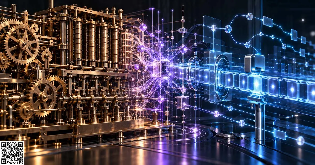
What does it mean for a machine to compute? Can mechanical components execute mathematical instructions without continuous human intervention? What distinguishes a specialized calculating device from a general-purpose programmable computer? Can one machine reproduce the operations of another machine merely by interpreting its instructions? Are there mathematical problems that no algorithm can solve, regardless of the available computing power? And how did the transformation from Charles Babbage’s nineteenth-century mechanical engines to Alan Turing’s twentieth-century mathematical theory of computation establish essential foundations for modern computers and artificial intelligence?

These questions concern computation, one of the most consequential concepts in mathematics, engineering, computer science, and the scientific investigation of intelligence.

Computation is the systematic transformation of information according to explicitly defined rules.

In its broad mathematical sense, computation can involve manipulating numbers, symbols, logical expressions, strings, graphs, representations, or other formally specified objects.

In practical engineering, computation is implemented through physical systems capable of representing information and carrying out prescribed operations.

The historical development of computation transformed calculation from a predominantly human activity into a process that could be automated, programmed, generalized, and eventually studied as a mathematical object in its own right.

Two particularly influential figures in this transformation were Charles Babbage (1791–1871) and Alan Mathison Turing (1912–1954).

Babbage developed designs for mechanical calculating engines and conceived an ambitious programmable machine known as the Analytical Engine.

His earlier Difference Engine was designed to automate the production of numerical tables through finite-difference methods.

The Analytical Engine introduced a substantially more general conception of machine computation.

Its proposed architecture distinguished numerical storage from arithmetic processing and used punched-card-controlled operations to describe computational procedures.

These ideas anticipated important characteristics of later programmable computers, although the Analytical Engine was never completed as a functioning general-purpose machine during Babbage’s lifetime [1][2].

Ada Lovelace (1815–1852), working in close intellectual collaboration with Babbage, made an exceptional contribution to the conceptual understanding of programmable computation.

Her extensive notes accompanying an 1843 translation of Luigi Federico Menabrea’s description of the Analytical Engine included a detailed tabulation of operations for calculating Bernoulli numbers.

More importantly, Lovelace recognized that a programmable machine might manipulate symbols representing entities other than numerical quantities.

Her observations anticipated an important principle of general-purpose computing:

A machine capable of manipulating representations according to formal rules need not be restricted to arithmetic as its ultimate application.

Yet the evolution of computation was not a direct, uninterrupted historical progression from Babbage and Lovelace to Turing.

Between their work and the development of modern computing, mathematicians, engineers, logicians, and inventors pursued partially independent investigations.

George Boole helped establish the algebraic foundations of symbolic logic.

Gottlob Frege developed formal logical systems capable of expressing mathematical relationships.

Georg Cantor, Giuseppe Peano, Bertrand Russell, David Hilbert, Kurt Gödel, Alonzo Church, Emil Post, Stephen Kleene, and others contributed to increasingly rigorous investigations of mathematical formalization, effective procedures, and the limits of deductive systems.

During the early twentieth century, problems concerning the foundations of mathematics gave rise to a fundamental question:

Can every precisely formulated mathematical problem be solved through a finite sequence of mechanical instructions?

Turing addressed this question in his landmark paper On Computable Numbers, with an Application to the Entscheidungsproblem, submitted in 1936 and published in 1937 [8].

He introduced an idealized model of computation now known as the Turing machine.

The model describes a device with a finite collection of internal states, a symbolic tape, a read–write mechanism, and rules determining the machine’s operations.

Despite its conceptual simplicity, this model provides a powerful mathematical representation of effective computation.

Turing also demonstrated the principle of universal computation: a suitably constructed universal machine can simulate the operations of other machines when supplied with their encoded descriptions and inputs.

This established a profound conceptual distinction between a machine dedicated to one specific procedure and a machine capable of executing descriptions of many different procedures.

Turing’s work also helped establish fundamental limitations of algorithmic computation.

Certain mathematical problems cannot be solved by any algorithm operating under the standard model of effective computation.

Thus, computation is not merely a question of building sufficiently powerful machinery.

It also concerns the mathematical boundaries of what systematic procedures can accomplish.

The subsequent history of electronic computing involved contributions from Konrad Zuse, John Atanasoff, Clifford Berry, Tommy Flowers, Howard Aiken, John Mauchly, J. Presper Eckert, John von Neumann, Maurice Wilkes, Frederic Williams, Tom Kilburn, Geoff Tootill, and many others.

The emergence of electronic stored-program computers established practical architectures in which instructions and data could be represented electronically and processed at high speed.

These developments ultimately made large-scale computational science and artificial intelligence technically feasible.

Modern artificial intelligence depends on computation at several interconnected levels.

Algorithms specify procedures for learning, searching, optimizing, reasoning, and generating outputs.

Programming languages express these procedures in executable forms.

Computer architectures implement the corresponding operations.

Computational complexity theory investigates the resources required to solve problems.

Computability theory determines whether problems admit algorithms at all.

Machine-learning systems use computational procedures to estimate parameters, process representations, and produce predictions.

Nevertheless, computational capability must not be confused with intelligence, consciousness, understanding, or factual reliability.

A universal computer can execute a remarkably broad class of formally specified procedures without automatically possessing humanlike comprehension.

A machine-learning system can perform complex computations while producing incorrect or misleading outputs.

An algorithm can be mathematically well defined while requiring impractical resources.

A computational system can implement its instructions correctly while pursuing an inappropriate objective.

Consequently, computation provides an indispensable foundation for artificial intelligence, but it does not independently establish every property associated with intelligent behavior.

This article examines the historical emergence of programmable calculation, Babbage’s mechanical computing designs, Lovelace’s conceptual contributions, Turing’s mathematical theory of computation, universal machines, undecidability, and the engineering development of electronic stored-program computers.

It also investigates the technical mechanics of computation, the formal structure of algorithms, computational complexity, and the relationship between computability and modern artificial intelligence.

Throughout, a central distinction is maintained:

Mechanical calculation, programmable computation, mathematical computability, and artificial intelligence are related but not identical concepts.

---

1. DEEP DEFINITION

1.1. What Is Computation?

Computation is the execution of a specified sequence of operations that transforms represented information according to defined rules.

A computational process ordinarily involves:

• Input representations.
• A finite description of applicable operations.
• A mechanism for selecting and executing those operations.
• Intermediate computational states.
• Rules governing state transitions.
• Output, termination, or continued execution.

A simple mathematical abstraction is:

Output = F(Input)

Where F represents the transformation performed by the computational procedure.

For a terminating deterministic algorithm, this may describe a mathematical function.

However, not every computational process terminates, and some computational systems are interactive, probabilistic, concurrent, or continuously supplied with new information.

Therefore, the simple function representation captures only part of the broader concept.

The theory of computation studies how such processes can be specified, implemented, compared, and mathematically analyzed.

1.2. Computation Versus Calculation

Calculation usually refers to evaluating numerical or mathematical expressions.

For example:

7 × 8 = 56

Computation is broader.

A machine may compute by:

• Sorting records.
• Comparing symbols.
• Verifying logical statements.
• Searching a graph.
• Processing an image.
• Encoding information.
• Executing a simulation.
• Generating a language sequence.
• Transforming a mathematical proof representation.

Arithmetic calculation is therefore a form of computation, but computation is not limited to arithmetic.

This distinction was central to the historical movement from specialized calculating devices toward general-purpose machines.

1.3. What Is an Algorithm?

An algorithm is a precisely specified procedure for carrying out a computational task.

A conventional terminating algorithm contains a finite description of operations that can be executed systematically.

Its instructions must be sufficiently definite to determine permissible computational steps.

For example, Euclid’s algorithm calculates the greatest common divisor of two nonnegative integers, not both zero.

An illustrative procedure is:

1. Receive integers a and b.

2. If b = 0, return a.

3. Otherwise, replace (a, b) with (b, a mod b).

4. Repeat until b = 0.

The procedure terminates for valid inputs and returns the greatest common divisor.

This example demonstrates that algorithms long predate electronic computers.

The historical contribution of programmable computing was not the invention of algorithms themselves.

It was the development of increasingly general mechanisms for executing them automatically.

1.4. Historical Algorithms Before Mechanical Computing

Algorithmic methods developed across multiple intellectual traditions.

Ancient Egyptian and Babylonian mathematics included systematic numerical procedures.

Greek mathematics developed constructive and deductive methods.

Euclid’s Elements contains a systematic procedure for finding greatest common divisors.

Mathematical traditions in India, China, and the Islamic world developed important arithmetic, algebraic, and computational procedures.

The term algorithm is historically associated with the Latinized name of the mathematician Muhammad ibn Musa al-Khwarizmi.

His ninth-century mathematical writings significantly influenced the transmission and development of arithmetic and algebraic methods.

These contributions established a long historical foundation for systematic computation.

Modern computation did not originate from a single European invention.

1.5. The Historical Role of Human Computers

Before electronic computing, the term computer commonly referred to a person engaged in mathematical calculation.

Human computers carried out numerical procedures for:

• Astronomy.
• Navigation.
• Engineering.
• Surveying.
• Ballistics.
• Insurance.
• Government statistics.
• Scientific research.

Large calculations were often divided into repeated operations carried out according to explicit instructions.

The work could be demanding, repetitive, and vulnerable to transcription or arithmetic errors.

Women played major roles in numerous human-computing organizations, particularly during the development of scientific and electronic computing.

The historical transition to machine computation involved automating operations previously performed by human calculators.

Turing’s mathematical analysis of computation was partly motivated by considering the elementary steps available to a human carrying out a systematic calculation.

1.6. Mechanical Calculation Before Babbage

Mechanical calculating devices existed long before Babbage.

Important historical examples include:

Blaise Pascal’s Pascaline

Developed during the 1640s, it used mechanical components to assist arithmetic calculation.

Gottfried Wilhelm Leibniz’s stepped-reckoner designs

These investigated mechanical implementations of arithmetic operations using stepped mechanisms.

Other calculating instruments

Slide rules, logarithmic tables, adding machines, and specialized mechanisms assisted scientific and commercial calculations.

Such devices automated particular operations.

However, a specialized arithmetic machine is not automatically a general-purpose programmable computer.

The distinction depends on the machine’s representation, control mechanisms, and ability to execute different procedures.

1.7. Joseph Marie Jacquard and Programmable Control

Joseph Marie Jacquard is associated with the development of a loom mechanism controlled through punched cards.

The punched-card mechanism allowed patterns to be represented externally and used to control mechanical operations.

A card’s pattern of holes influenced how the machine operated.

This was an important example of externally specified machine control.

However, a programmable textile loom should not automatically be described as a general-purpose computer.

Its programming capability concerned a specialized manufacturing process.

The broader historical significance lies in demonstrating how mechanical behavior could be controlled through encoded instructions.

This principle influenced Babbage’s Analytical Engine design [2].

1.8. Charles Babbage and the Problem of Mathematical Tables

Charles Babbage was a British mathematician and inventor whose work fundamentally influenced the conception of automated computation.

During the early nineteenth century, scientists and engineers depended heavily on printed numerical tables.

Such tables were used for:

• Astronomy.
• Navigation.
• Surveying.
• Engineering.
• Mathematical analysis.
• Insurance.
• Financial calculation.

Producing these tables required substantial human effort.

Errors could arise during calculation, transcription, typesetting, or printing.

Babbage investigated how mechanical systems could automate the generation of tables and reduce certain categories of human error.

His work eventually led to the Difference Engine and Analytical Engine concepts.

1.9. Babbage’s Difference Engine

The Difference Engine was designed to calculate and tabulate values of mathematical functions using the method of finite differences.

Babbage publicly described an early Difference Engine concept in 1822.

Work on a larger machine began in the following years.

Its principal purpose was to automate numerical table production.

Instead of requiring a general-purpose arithmetic system capable of evaluating every formula directly, a difference engine could exploit mathematical relationships among successive values.

For polynomial functions, repeated finite differences eventually become constant.

A machine could therefore generate a sequence of values through repeated additions.

This was a major application of mathematical structure to mechanical calculation [1][3].

1.10. Finite Differences

For a function f evaluated at consecutive integer arguments, the first forward difference is:

Δf(x) = f(x + 1) − f(x)

The second difference is:

Δ²f(x) = Δf(x + 1) − Δf(x)

Higher differences are defined recursively:

Δᵏ⁺¹f(x) = Δ(Δᵏf(x))

For a polynomial of degree d with equally spaced inputs, the d-th forward difference is constant.

Differences of order greater than d are zero in exact arithmetic.

This property makes repeated addition sufficient for generating polynomial tables.

1.11. Worked Example: Generating Squares

Consider:

f(x) = x²

For x = 0, 1, 2, 3, 4:

x	f(x)	First difference	Second difference
0	0	1	2
1	1	3	2
2	4	5	2
3	9	7	2
4	16	—	—

The first differences are:

1, 3, 5, 7

The second differences are:

2, 2, 2

Therefore, a machine can generate the squares using additions.

Starting with:

Value = 0

First difference = 1

Second difference = 2

At each step:

Next value = Current value + First difference

Next first difference = Current first difference + Second difference

This produces:

0, 1, 4, 9, 16, …

The calculation illustrates the mathematical principle behind a difference engine.

It does not reproduce every mechanical detail of Babbage’s engineering designs.

1.12. The Difference Engine’s Mechanical Architecture

Babbage’s Difference Engine designs used interconnected mechanical components to represent numerical values and perform arithmetic operations.

Their conceptual architecture included:

• Number storage in mechanical digit columns.
• Addition mechanisms.
• Carry propagation.
• Repeated operation cycles.
• Mechanisms associated with producing numerical results.

The machine was intended to reduce the manual calculations required for generating tables.

However, its architecture was specialized.

It was not designed to execute arbitrary user-supplied algorithms in the manner envisioned for the later Analytical Engine.

1.13. Why the Original Difference Engine Was Not Completed

Babbage encountered substantial engineering and financial challenges.

These included:

• Difficulties in precision manufacturing.
• Large component requirements.
• Project-management problems.
• Disagreements with engineering collaborators.
• Financial and governmental constraints.
• Changing design ambitions.

A working demonstration section was constructed, but the full original engine was not completed during Babbage’s lifetime.

The project nevertheless influenced subsequent developments in mechanical computing [1].

Its incompletion should not be interpreted as proof that the underlying mathematical principles were invalid.

1.14. Difference Engine No. 2

Babbage later developed a revised Difference Engine design.

Difference Engine No. 2 was conceived during the 1840s.

It incorporated engineering simplifications compared with earlier proposals.

A complete machine based on Babbage’s historical design was eventually constructed through a modern museum engineering project.

The Computer History Museum documents the construction and operation of Difference Engine No. 2.

The successful modern realization provides important evidence that the historical design could operate when manufactured and assembled appropriately [1].

However, modern construction does not mean that the machine was completed in the nineteenth century.

1.15. From Specialized Calculation to Programmable Computation

The Difference Engine addressed a comparatively restricted category of numerical procedures.

Babbage subsequently conceived a machine capable of performing a broader range of calculations through instructions supplied in advance.

This became the Analytical Engine.

The conceptual transformation was significant.

Instead of constructing a separate machine for each numerical procedure, Babbage proposed a machine whose operations could be varied through an external program.

The machine’s physical mechanism would remain broadly the same while its instructions changed.

This principle anticipated general-purpose programmable computing.

1.16. The Analytical Engine

Babbage began developing the Analytical Engine concept during the 1830s.

The proposed machine was intended to manipulate numerical values through a sequence of programmed operations.

Important architectural elements included:

The Store

A mechanism for retaining numbers and intermediate results.

The Mill

A mechanism for carrying out arithmetic operations.

Punched-card control

An approach for specifying operations and directing the machine’s behavior.

Control mechanisms

Proposed procedures for managing the order of operations and repeating computational sequences.

Output mechanisms

Methods for producing or recording results.

The design introduced a conceptual separation between storage, processing, and instruction-controlled execution.

This separation remains recognizable in later computer architectures [1][2].

1.17. The Store and the Mill

The Analytical Engine’s Store was conceptually similar to a memory system holding values.

The Mill was conceptually similar to a computational processing unit.

The Store retained numbers.

The Mill performed arithmetic operations on numbers supplied to it.

Intermediate results could be returned to storage.

This relationship can be represented as:

Store → Mill → Store

The analogy with modern memory and processors is useful.

However, the Analytical Engine’s proposed mechanisms were mechanical and decimal, not identical to modern electronic binary processors.

1.18. Punched Cards and Program Representation

The Analytical Engine was designed to use punched cards for controlling operations.

Babbage considered different card roles associated with operations and variables.

This allowed the machine’s computational behavior to be represented separately from its physical arithmetic mechanisms.

The distinction is fundamental.

A machine’s hardware can remain unchanged while its instructions specify different sequences of operations.

However, externally supplied punched-card instructions are not identical to electronically stored programs.

The historical distinction between external program media and instructions stored in writable electronic memory must be preserved.

1.19. Repetition and Conditional Control

The Analytical Engine’s design incorporated concepts associated with repeated computational sequences and conditional operation.

Such mechanisms are important because many algorithms require their next step to depend on earlier results.

For example:

If a computed quantity satisfies a specified condition, execute one sequence; otherwise, execute another.

Similarly, repeated operations can be performed through a control structure resembling a loop.

The precise mechanical realization of these concepts must be distinguished from modern programming-language syntax.

Babbage did not design a contemporary Python interpreter or electronic instruction processor.

Nevertheless, his work anticipated important ideas in machine-controlled algorithm execution.

1.20. Luigi Federico Menabrea and the Analytical Engine

Luigi Federico Menabrea published a description of Babbage’s Analytical Engine in French in 1842.

The article was based on information associated with Babbage’s presentations in Turin.

Menabrea’s account helped explain the machine’s proposed architecture and operations.

Ada Lovelace subsequently translated the article into English and appended extensive notes.

The combined publication became one of the most historically important documents concerning the Analytical Engine.

1.21. Ada Lovelace and the Mathematical Interpretation of Programming

Ada Lovelace was a mathematician whose contribution to the history of computation extended beyond the description of an individual calculating procedure.

Her 1843 publication included detailed explanations of the Analytical Engine’s possible operations.

The notes demonstrated how computational processes could be systematically represented.

One notable example concerned the calculation of Bernoulli numbers.

Lovelace’s work is frequently associated with the earliest published computer programs.

However, the exact designation of the world’s first programmer is historically debated because Babbage had developed unpublished computational procedures and the two collaborated closely.

The strongest historically defensible conclusion is that Lovelace made a substantial, documented contribution to early programming concepts and published a particularly influential representation of a computational procedure [4][5].

1.22. Lovelace’s Bernoulli-Number Example

Bernoulli numbers form an important mathematical sequence.

They appear in number theory, series expansions, and mathematical analysis.

A standard generating-function definition is:

t / (eᵗ − 1) = Σₙ₌₀∞ Bₙtⁿ / n!

Under this convention:

B₀ = 1

B₁ = −1/2

B₂ = 1/6

B₃ = 0

B₄ = −1/30

Lovelace’s Note G included a tabular representation of operations intended for an Analytical Engine calculation involving Bernoulli numbers.

Its significance lies in the explicit organization of variables, operations, and intermediate values.

The historical table should not be treated as identical to a program written in a modern programming language.

1.23. Lovelace and Symbolic Manipulation

Lovelace recognized that machine operations could potentially apply to symbols representing more than numerical quantities.

For example, numerical encodings could represent musical relationships or other formal structures.

This observation anticipated a fundamental principle of general-purpose computing:

The same computational machinery can manipulate different kinds of information when those kinds of information are represented through suitable symbols and rules.

Modern computers represent text, images, audio, and numerical data through encoded structures.

The physical operations of a processor do not intrinsically distinguish whether a bit pattern represents a number, character, pixel, or machine instruction.

The interpretation depends on the computational system.

Lovelace’s analysis was historically important because it articulated possibilities extending beyond conventional numerical calculation [4][5].

1.24. The Limits of Lovelace’s Claims

Lovelace also distinguished executing specified operations from independently originating arbitrary intellectual ideas.

This observation later became influential in philosophical discussions of machine intelligence.

However, it should not be simplified into a definitive proof that computers can never generate novel or unexpected results.

Modern computational systems can produce outputs that were not individually anticipated by their designers.

Whether such outputs constitute creativity, understanding, or autonomous intellectual originality is a separate philosophical and scientific question.

Lovelace’s historical arguments must be interpreted within the computational capabilities and conceptual debates of her period.

1.25. Herman Hollerith and Punched-Card Data Processing

Herman Hollerith developed electromechanical punched-card tabulation technology during the late nineteenth century.

His systems were notably used in processing the United States census of 1890.

Punched cards represented information that could be processed by machines.

This development demonstrated the practical value of machine-readable data representation.

It also contributed to the growth of commercial data-processing technologies.

However, Hollerith’s early tabulators were not identical to universal programmable computers.

They belonged to an important but distinct technological lineage.

1.26. Boolean Logic and Computation

George Boole’s mathematical investigations helped establish algebraic methods for representing logical relationships.

Boolean operations include:

AND

OR

NOT

These operations later became central to switching-circuit theory and digital computing.

For binary values:

A ∧ B

evaluates to one only when both inputs are one.

A ∨ B

evaluates to one when at least one input is one.

¬A

reverses a Boolean truth value.

The connection between Boolean logic and physical switching systems became especially significant through Claude Shannon’s twentieth-century work [13].

This mathematical lineage was important but historically distinct from Babbage’s mechanical computing designs.

1.27. Gottlob Frege and the Formalization of Mathematical Reasoning

Gottlob Frege’s 1879 Begriffsschrift introduced an influential formal language for representing quantification, functions, and logical relationships.

Frege’s work contributed to the broader mathematical movement toward explicit symbolic representation.

Formalized reasoning made it possible to investigate precisely which conclusions follow from particular axioms and inference rules.

This development helped create the intellectual environment in which computability could eventually be studied mathematically.

However, Frege’s historical contributions concerned mathematical logic rather than the engineering design of electronic computers.

1.28. David Hilbert and the Decision Problem

David Hilbert’s program sought rigorous foundations for mathematics.

A major question associated with mathematical logic was whether a general procedure could determine the validity of arbitrary formulas in a suitable formal system.

The Entscheidungsproblem, or decision problem, was prominently formulated in Hilbert and Wilhelm Ackermann’s 1928 work.

In modern terms, the question asks whether an algorithm can decide the validity of every formula in unrestricted first-order logic.

This question was essential to the development of computability theory.

Answering it required a sufficiently precise mathematical understanding of what counts as an algorithm.

1.29. Kurt Gödel and the Limits of Formal Systems

Kurt Gödel’s 1931 incompleteness results established profound limitations concerning sufficiently expressive formal theories [6].

Under appropriate conditions, an effectively axiomatized, consistent theory capable of representing enough arithmetic cannot prove every sentence expressible in its language.

Gödel’s work also demonstrated the power of encoding syntactic expressions and proofs numerically.

This technique is commonly associated with Gödel numbering.

The encoding of symbolic structures into numbers became important to computability theory.

However, Gödel’s incompleteness theorems should not be confused with Turing’s undecidability results.

They concern different mathematical properties, even though the developments are closely connected.

1.30. Alonzo Church and Lambda-Definability

Alonzo Church investigated the mathematical foundations of effective calculation.

His work introduced and developed formal systems involving lambda calculus and related concepts of definability.

In 1936, Church published research demonstrating the unsolvability of an important class of mathematical problems [7].

Lambda calculus describes computation through function abstraction and application.

It provides a mathematically different representation from Turing’s tape-based model.

Nevertheless, the classes of effectively computable numerical functions represented by the standard formulations were subsequently shown to coincide.

This equivalence became central to the modern understanding of computability.

1.31. Emil Post and Finite Combinatory Processes

Emil Post independently investigated formal models of symbolic computation.

His 1936 paper:

Finite Combinatory Processes—Formulation 1

presented a mathematical model involving symbol spaces and fixed instructions [9].

Post’s formulation shared important characteristics with Turing’s work.

Both addressed the possibility of describing computational procedures through simple symbolic operations.

These developments demonstrate that the mathematical concept of effective computation emerged through multiple independent lines of research.

1.32. Alan Turing and the Mathematical Definition of Computation

Alan Turing introduced his abstract computing-machine model in a paper submitted in 1936 and published in 1937 [8].

Turing investigated the elementary operations involved in following a mechanical procedure.

His idealized machine contained:

• A tape divided into discrete cells.
• A finite alphabet of symbols.
• A read–write head.
• A finite collection of internal states.
• A transition rule.

The machine could inspect a symbol, write another symbol, change its internal state, and move along the tape.

By combining these simple operations, complex computations could be represented.

The significance was mathematical rather than primarily mechanical.

Turing was establishing a formal model of effective computation, not presenting construction plans for a specific electronic device.

1.33. The Turing Machine

A standard deterministic Turing machine can be described through a tuple:

M = (Q, Σ, Γ, δ, q₀, qₐ, qᵣ)

Where:

• Q is a finite set of states.
• Σ is the input alphabet.
• Γ is the tape alphabet.
• δ is the transition function.
• q₀ is the initial state.
• qₐ is an accepting state.
• qᵣ is a rejecting state.

The precise formal definition varies slightly across textbooks.

A transition may be represented as:

δ(q, a) = (q′, b, D)

Where:

• q is the current state.
• a is the scanned symbol.
• q′ is the next state.
• b is the symbol written.
• D is the direction of head movement.

Despite the model’s simple operations, Turing machines can represent an exceptionally broad class of algorithms.

1.34. Universal Computation

Turing’s work introduced the concept of a universal machine.

A universal Turing machine can simulate other Turing machines when supplied with their encoded descriptions and inputs.

Symbolically:

U(⟨M⟩, x) = M(x)

whenever the simulated computation produces a defined result.

Here:

• U is the universal machine.
• ⟨M⟩ is an encoding of another machine.
• x is the input supplied to M.

The result means that one fixed computational mechanism can implement many different procedures.

Universality is a defining mathematical idea behind general-purpose programmable computing.

However, the original universal Turing machine is an abstract mathematical construction.

It is not the same thing as a physically realizable computer with unlimited memory.

1.35. The Church–Turing Thesis

The Church–Turing thesis proposes that every effectively calculable function can be computed by a Turing machine.

The thesis links an informal notion—effective calculation—to a precisely defined mathematical model.

Different formal approaches, including Turing machines and lambda calculus, characterize the same class of standard computable numerical functions.

However, the Church–Turing thesis is not a conventional theorem proved from a fully formal definition of all possible effective procedures.

Its central claim concerns the relationship between formal models and an informal concept [10].

This distinction is essential.

The thesis should not be misrepresented as proof that all physical phenomena are computable or that every conceivable form of intelligence is Turing-computable.

1.36. Turing and the Entscheidungsproblem

Turing used his mathematical model to investigate the possibility of general algorithms for mathematical decision problems.

His work established results connected to the impossibility of a universal decision procedure for unrestricted first-order logical validity.

Church independently established an unsolvability result through a different formal approach.

These results answered the Entscheidungsproblem negatively.

There is no algorithm that correctly decides the validity of every arbitrary first-order formula and always terminates.

The result does not mean that practical automated theorem proving is impossible.

Many logical problems and restricted fragments remain decidable.

1.37. Undecidability and the Halting Problem

A central result in computability theory concerns the halting problem.

The problem asks whether there exists an algorithm that, given an arbitrary program and input, always determines whether the program will terminate.

The general halting problem is undecidable.

There is no algorithm that correctly answers this question for every possible program-input pair and always terminates.

This limitation is mathematical.

It does not arise merely because existing computers are too slow.

1.38. Computation Versus Computational Complexity

Computability asks whether a problem admits an algorithm.

Computational complexity asks how many resources are required to execute an algorithm.

These are distinct questions.

A problem may be decidable but computationally expensive.

For example, an exhaustive search algorithm may eventually solve every instance of a finite problem but require resources growing exponentially with input size.

Conversely, an undecidable problem has no general terminating decision algorithm under the standard model.

Increasing processor speed cannot remove that mathematical limitation.

1.39. Konrad Zuse and Early Programmable Machines

Konrad Zuse designed and constructed early computing machines in Germany.

His Z3, completed in 1941, was an important electromechanical programmable digital computer.

Zuse’s work contributed to practical machine architectures using binary representations and automated arithmetic.

However, historical claims about the first computer depend on which criteria are being applied:

• Programmability.
• Generality.
• Electronic implementation.
• Digital representation.
• Stored-program operation.
• Actual construction.
• Successful execution.

No single historical label captures every dimension.

1.40. Colossus and Electronic Computing

Colossus machines were developed in Britain during the Second World War for specialized cryptanalytic operations.

Tommy Flowers played a major engineering role.

Colossus demonstrated the practical power of high-speed electronic digital processing.

However, Colossus was designed for specialized tasks and was not a general-purpose stored-program computer in the modern sense.

Its historical contribution must be evaluated according to its actual architecture and operational purpose.

1.41. ENIAC and General-Purpose Electronic Calculation

ENIAC was developed in the United States by a team including John Mauchly and J. Presper Eckert.

It became operational during the 1940s.

ENIAC was a major early general-purpose electronic digital computer.

Its original programming arrangements involved switches and cable connections rather than the later conventional approach of keeping executable instructions in general electronic memory.

Its design demonstrated the feasibility of high-speed electronic computation on a large scale.

1.42. John von Neumann and Stored-Program Architecture

John von Neumann’s 1945 First Draft of a Report on the EDVAC presented an influential description of electronic computing architecture [14].

The report discussed how computational systems could organize:

• Arithmetic operations.
• Control.
• Memory.
• Input.
• Output.

It became strongly associated with stored-program computer architecture.

However, the conceptual and engineering development of stored-program computers involved multiple contributors.

The widespread label von Neumann architecture should not be interpreted as assigning sole historical invention to von Neumann.

1.43. The Manchester Baby and Electronic Stored Programs

The Manchester Small-Scale Experimental Machine, commonly known as the Manchester Baby, successfully executed a program stored electronically in its memory on 21 June 1948.

The machine was developed through work involving Frederic Williams, Tom Kilburn, and Geoff Tootill.

Its purpose included testing electronic memory technology.

The successful execution of a stored program was a major engineering milestone.

It demonstrated that instructions could be retained electronically and executed by an electronic digital machine [16].

1.44. Alan Turing and Machine Intelligence

Turing’s contribution extended beyond the mathematical study of computable functions.

In 1950, he published:

Computing Machinery and Intelligence

in the journal Mind [17].

The paper introduced an influential discussion of machine intelligence through the imitation game.

Turing investigated whether machine behavior could be evaluated through an operationally specified conversational test.

His discussion influenced later artificial intelligence research.

However, success in an imitation-game-style evaluation does not independently establish consciousness, subjective experience, or comprehensive understanding.

The mathematical concept of universal computation and the philosophical evaluation of intelligence are distinct.

1.45. Historical Development Timeline

Year	Development	Significance
Ancient period	Systematic mathematical algorithms across multiple civilizations	Foundations of rule-governed calculation
Ninth century	Al-Khwarizmi’s mathematical writings	Influential development and transmission of algorithmic methods
1640s	Pascal develops mechanical calculator	Mechanization of arithmetic
Seventeenth century	Leibniz develops calculating mechanisms	Expansion of mechanical arithmetic
Early nineteenth century	Jacquard punched-card-controlled loom	External encoding of machine operations
1822	Babbage announces Difference Engine work	Automated numerical table calculation
1823	Major Difference Engine construction begins	Attempted large-scale precision mechanical computing
1830s	Babbage develops Analytical Engine concept	General-purpose programmable mechanical computation
1842	Menabrea publishes Analytical Engine description	Technical dissemination of Babbage’s design
1843	Lovelace publishes translation and extensive notes	Early published program description and symbolic computation concepts
1854	Boole publishes The Laws of Thought	Mathematical foundations of logical operations
1879	Frege publishes Begriffsschrift	Advanced formal logical representation
1890	Hollerith punched-card tabulation used in U.S. census	Large-scale electromechanical data processing
1900	Hilbert presents mathematical research problems	Formal foundational research agenda
1928	Hilbert and Ackermann formulate the decision problem prominently	Search for general logical decision procedures
1931	Gödel publishes incompleteness results	Fundamental limitations of formal theories
1936	Church publishes unsolvability research	Formal limits of effective calculation
1936	Post publishes finite combinatory-process model	Independent mathematical model of computation
1936–1937	Turing develops and publishes computability theory	Turing machines, universality, and undecidability
1938	Shannon publishes switching-circuit analysis	Boolean mathematics connected with electrical switching
1941	Zuse’s Z3 operates	Electromechanical programmable digital computation
1943–1944	Colossus machines developed and deployed	Specialized electronic digital processing
1945	Von Neumann’s EDVAC report circulated	Influential stored-program architecture description
1946	ENIAC publicly demonstrated	Large-scale electronic digital computation
1948	Manchester Baby executes stored program	Electronic stored-program milestone
1949	EDSAC begins regular computing operations	Practical stored-program computing service
1950	Turing publishes Computing Machinery and Intelligence	Influential operational discussion of machine intelligence
1971	Cook establishes foundational complexity results	NP-completeness and complexity theory
Later twentieth century	Microprocessors, networks, and software ecosystems expand	Broad deployment of programmable computation
Contemporary era	Large-scale AI and accelerator-based computation	Massive parallel processing of learned models

The chronology summarizes selected developments.

It does not imply that every later computer was directly derived from Babbage’s designs or Turing’s original paper.

---

2. TECHNICAL MECHANICS

2.1. The Fundamental Components of Computation

A computational system can be analyzed through several conceptual components.

Representation

How information is encoded.

State

The currently retained computational information.

Operations

The actions the system can perform.

Control

The rules determining which action occurs next.

Memory

The mechanism for preserving information.

Output

The result of computation, when a result is produced.

These components may be implemented through mechanical, electronic, or abstract mathematical mechanisms.

2.2. Mathematical Functions and Computation

A numerical function can be represented as:

f: X → Y

Where:

• X is the input domain.
• Y is the output domain.
• f maps each valid input to its output.

A computational procedure implements f when it produces the appropriate result for inputs in its specified domain.

However, not every mathematically defined function is computable.

Furthermore, programs can represent partial functions.

A partial function may be undefined for some inputs because the corresponding computation does not terminate.

2.3. Deterministic Computational Procedures

A deterministic computational procedure has a specified next operation for every relevant state and input.

A transition can be represented as:

Sₜ₊₁ = F(Sₜ)

Where Sₜ is the current computational state.

For a deterministic system, the same initial configuration produces the same sequence of states, assuming identical execution semantics.

This does not mean the system necessarily terminates.

A deterministic program can enter an infinite loop.

2.4. State Machines

A finite-state machine contains a finite collection of states and rules governing transitions.

A deterministic finite automaton is commonly represented as:

A = (Q, Σ, δ, q₀, F)

Where:

• Q is a finite state set.
• Σ is an input alphabet.
• δ is a transition function.
• q₀ is the initial state.
• F is a set of accepting states.

Finite automata are important for recognizing regular languages.

However, ordinary finite automata lack unrestricted read–write memory.

They are therefore less computationally expressive than Turing machines.

2.5. Mechanical Representation of Numerical Values

Babbage’s machines represented numerical quantities through mechanical digit mechanisms.

In a decimal mechanical representation, a wheel or column may represent a digit from zero through nine.

Multiple positions together represent larger numbers.

For example:

438 = 4 × 10² + 3 × 10¹ + 8 × 10⁰

Mechanical operations must account for changes in individual digit positions.

A carry operation occurs when addition exceeds the current digit’s capacity.

2.6. Mechanical Addition

Consider:

478 + 56

Column arithmetic gives:

8 + 6 = 14

Write four in the units position and carry one.

Then:

7 + 5 + 1 = 13

Write three in the tens position and carry one.

Finally:

4 + 1 = 5

The result is:

534

A mechanical calculator must implement equivalent positional operations through physical movement.

Carry propagation is therefore a central engineering concern.

2.7. Finite-Difference Computation

Let:

f(n) = n²

Then:

Δf(n) = 2n + 1

and:

Δ²f(n) = 2

Therefore, a sequence of square values can be generated without direct multiplication at every step.

A conceptual implementation maintains:

Value

FirstDifference

SecondDifference

The update rules are:

Value ← Value + FirstDifference

FirstDifference ← FirstDifference + SecondDifference

The second difference remains constant.

This is the algorithmic structure behind the example of mechanical finite-difference calculation.

2.8. Polynomial Computation Through Finite Differences

For a polynomial of degree d:

f(n) = a₀ + a₁n + … + aₙnᵈ

with the final coefficient indexed appropriately as a_d, its forward differences of order d are constant.

Using the corrected conventional expression:

f(n) = Σₖ₌₀ᵈ aₖnᵏ

the d-th difference is constant for unit-spaced arguments.

The difference table can be updated using additions.

This makes the method valuable for mechanical tabulation.

However, functions that are not polynomials generally require approximation or alternative representations.

2.9. The Difference Engine’s Operational Cycle

A conceptual difference-engine cycle is:

1. Retain the current function value.

2. Retain successive finite differences.

3. Add the next difference to the current value.

4. Update the stored differences.

5. Produce the next table entry.

6. Repeat.

The machine’s particular mechanical timing and carry mechanisms determine how these operations are physically coordinated.

2.10. Numerical Approximation

Difference engines could generate tables for functions represented or approximated by polynomials.

Suppose a function g(x) is approximated near a point a by a polynomial:

g(x) ≈ Pₙ(x)

A Taylor polynomial is one possible representation:

Pₙ(x) = Σₖ₌₀ⁿ [g⁽ᵏ⁾(a)/k!](x − a)ᵏ

If a suitable approximation is constructed, finite-difference methods can generate its values.

The quality of the resulting numerical table depends on the approximation and arithmetic precision.

A mechanically accurate calculation of an inadequate approximation can still produce inaccurate results.

2.11. The Analytical Engine’s Store

The Store was intended to retain numerical quantities and intermediate computational results.

This is conceptually related to memory in modern computing.

A stored number could be retrieved for arithmetic processing.

The result could then be returned to storage.

However, the Store was a proposed mechanical system.

It should not be equated literally with semiconductor random-access memory.

2.12. The Analytical Engine’s Mill

The Mill was designed to carry out arithmetic operations.

A general computation could involve:

Read operands from storage.

Perform arithmetic.

Write the result to storage.

This is conceptually similar to a processor’s interaction with memory.

However, Babbage’s design used mechanical decimal operations rather than electronic binary logic.

2.13. Instruction-Controlled Computation

A programmed machine must represent which operation to perform.

A conceptual instruction may contain:

Operation

Operand locations

Destination location

For example:

ADD A, B → C

means to add the values represented by A and B and store the result in C.

This is modern explanatory notation, not a literal reconstruction of Babbage’s card format.

Its purpose is to illustrate how instructions can separate computational behavior from machine hardware.

2.14. Program Sequences

A program may consist of ordered instructions.

For example:

Load A

Load B

Add

Store C

Output C

The sequence defines a computational procedure.

Changing the instructions can change the procedure without requiring a completely different arithmetic mechanism.

This property is central to general-purpose programmability.

2.15. Conditional Branching

Conditional branching changes the instruction sequence according to a computed condition.

A conceptual example is:

If x ≥ 0, return x. Otherwise, return −x.

This computes an absolute value.

Mathematically:

|x| = x if x ≥ 0

|x| = −x if x < 0

Branching allows programs to respond to intermediate computational states.

Without conditional control, many algorithms would be difficult or impossible to express efficiently in their usual forms.

2.16. Iteration

Iteration repeats a sequence of operations.

For example, the factorial of a nonnegative integer n is:

n! = ∏ₖ₌₁ⁿ k

with:

0! = 1

An iterative algorithm initializes an accumulator and repeatedly multiplies by successive integers.

Iteration provides a way to express repetitive computation through a finite program.

A loop must have appropriate termination conditions when termination is required.

2.17. Recursion

Recursion defines a procedure in terms of smaller instances of a related problem.

For example:

Factorial(0) = 1

Factorial(n) = n × Factorial(n − 1)

for positive integer n.

A recursive implementation must manage intermediate calls and state.

Recursion does not automatically imply efficient execution.

Its resource requirements depend on the algorithm and implementation.

2.18. Data Encoding

General-purpose computers manipulate encoded information.

A binary digit, or bit, can represent:

0

or:

1

A sequence of n bits has:

2ⁿ possible bit patterns

For example, eight bits provide:

2⁸ = 256 possible patterns

These patterns may encode numbers, characters, instructions, or other information.

The mathematical meaning of a bit pattern depends on the representation system.

2.19. Symbols Versus Their Encodings

Suppose a system assigns:

A → 65

under a particular character encoding.

The numerical value 65 is not inherently the letter A.

It acquires that interpretation through an encoding convention.

Likewise, a sequence of bytes can represent an image, text, audio data, or executable instructions.

This illustrates the general computational principle anticipated by Lovelace’s analysis of symbolic operations.

2.20. Boolean Computation

Binary hardware can implement logical operations.

For input bits a and b:

AND(a, b) = 1 only when a = 1 and b = 1

OR(a, b) = 1 when at least one input equals 1

NOT(a) = 1 − a

for a ∈ {0, 1}.

More complex logic functions can be constructed from simpler gates.

In particular, NAND is functionally complete under ordinary Boolean semantics.

This means that every Boolean function can be represented through an appropriate network of NAND operations.

2.21. Claude Shannon and Switching-Circuit Theory

Claude Shannon’s 1938 paper demonstrated the mathematical relationship between Boolean algebra and relay-switching circuits [13].

Logical expressions could be mapped to switching configurations.

For example:

Y = A ∧ B

corresponds to an output condition requiring both logical inputs.

This relationship became foundational to digital circuit design.

However, the physical implementation of Boolean logic requires attention to electrical timing, noise margins, and component limitations.

2.22. Formal Definition of a Turing Machine

A common deterministic Turing machine model contains:

M = (Q, Σ, Γ, δ, q₀, qₐ, qᵣ)

The transition function is:

δ: (Q − {qₐ, qᵣ}) × Γ → Q × Γ × {L, R}

for one conventional formulation.

Some variants permit a stationary head movement.

The machine repeatedly:

Reads the current tape symbol.

Consults the transition rule.

Writes a symbol.

Changes its internal state.

Moves the tape head.

The process continues until an appropriate halting state is reached or the computation proceeds indefinitely.

2.23. The Tape

A Turing machine’s tape consists of discrete cells.

Each cell contains a symbol from the tape alphabet.

The theoretical model ordinarily permits an unbounded supply of blank cells.

This is an idealization.

A physical computer does not possess infinite memory.

The unbounded tape is used to analyze computation without imposing an arbitrary fixed memory limit.

2.24. The Read–Write Head

The read–write head accesses one tape cell at a time.

Its operations may include:

Reading a symbol.

Replacing a symbol.

Moving left.

Moving right.

The head’s current location is part of the complete computational configuration.

The machine’s next action depends on the scanned symbol and internal state.

2.25. Internal States

A Turing machine has a finite set of internal states.

For example:

Q = {q₀, q₁, q₂, qAccept, qReject}

States represent different stages of the computational procedure.

The machine does not require an infinite collection of states.

Its unbounded computational potential comes from combining finite control with an unbounded tape.

2.26. The Transition Function

The transition function specifies an action for each relevant state-symbol pair.

For example:

δ(q₀, 1) = (q₀, 1, R)

This instructs the machine to:

• Remain in state q₀.
• Write the symbol 1.
• Move right.

Another rule may be:

δ(q₀, □) = (qAccept, 1, R)

where □ represents a blank symbol.

This rule writes one and enters an accepting state.

2.27. Worked Example: Unary Increment

Suppose an integer n is represented by n consecutive occurrences of the symbol 1.

For example:

111

represents three.

A unary increment machine should produce:

1111

representing four.

The procedure is:

1. Start at the leftmost input symbol.

2. Move right while reading 1.

3. When a blank is reached, write 1.

4. Halt.

Using transition rules:

δ(qScan, 1) = (qScan, 1, R)

δ(qScan, □) = (qAccept, 1, R)

The machine computes the successor function:

f(n) = n + 1

This example illustrates how a simple mathematical function can be implemented through elementary symbolic operations.

2.28. Computational Configurations

A complete Turing-machine configuration includes:

Current internal state.

Tape contents.

Head position.

The transition function transforms one configuration into another.

Symbolically:

Cₜ → Cₜ₊₁

The full execution is a sequence:

C₀ → C₁ → C₂ → …

A terminating computation eventually reaches a halting configuration.

A nonterminating computation continues indefinitely.

2.29. Machine Acceptance and Rejection

For a language-recognition problem, a Turing machine may halt in either an accepting or rejecting state.

A string is accepted when the machine enters its accepting state.

It is rejected when the machine enters its rejecting state.

However, a general Turing machine may fail to halt on some inputs.

Therefore, recognition and decision must be distinguished.

2.30. Decidable Languages

A language L is decidable when there exists a Turing machine that:

Accepts every string in L.

Rejects every string not in L.

Halts on every input.

Such a machine is a decider.

Decidability establishes the existence of a general terminating procedure.

It does not establish that the procedure is computationally efficient.

2.31. Turing-Recognizable Languages

A language is Turing-recognizable when a machine accepts every string belonging to it.

For strings outside the language, the machine may reject or run indefinitely.

A recognizable language is therefore not necessarily decidable.

This distinction is fundamental to computability theory.

A language is decidable if both it and its complement are Turing-recognizable.

2.32. Encoding a Machine as Data

A Turing machine has a finite description.

Its states, symbols, and transition rules can therefore be encoded as a finite string.

Let:

⟨M⟩

denote the encoding of machine M.

A pair consisting of a machine and input can also be encoded:

⟨M, x⟩

This allows the description of one machine to become data processed by another machine.

The encoding principle is central to universal computation.

2.33. Universal Turing Machines

A universal Turing machine U receives:

An encoded machine description ⟨M⟩

and:

Input x

It then simulates the operation of M on x.

Symbolically:

U(⟨M⟩, x) ≃ M(x)

The symbol ≃ indicates agreement of computational behavior under the chosen formal interpretation.

If M halts with a specified output, U can reproduce that output.

If M does not halt, the corresponding universal simulation does not halt.

The general mechanism does not need to be redesigned for every simulated machine.

2.34. Universality Versus a Specialized Machine

A specialized calculator performs a restricted set of operations.

A universal machine can interpret representations of many different programs.

However, universality is a mathematical property of the computational model.

A physically constructed computer has finite memory, finite energy, finite precision, and finite operational time.

Therefore, physical general-purpose programmability should not be identified without qualification with ideal mathematical universality.

2.35. Effective Computability

An effectively computable function is informally understood as one whose values can be obtained through a systematic finite procedure.

A formal model makes the relevant operations explicit.

Under the Church–Turing thesis:

Effectively calculable functions correspond to Turing-computable functions.

This correspondence is supported by the convergence of multiple formal models of computation.

However, the thesis is not a claim about every physically conceivable process.

2.36. Lambda Calculus

Lambda calculus expresses computation through abstraction and function application.

A function can be represented as:

λx.x + 1

This example is explanatory notation using arithmetic as an abbreviation for an appropriate formal encoding.

The expression represents a transformation mapping an input x to x + 1.

Function application may be written:

(λx.x + 1) 4

which reduces to:

5

In pure lambda calculus, numbers and arithmetic are represented through formal encodings rather than assumed as primitive operations.

Lambda calculus is central to programming-language theory and functional computation.

2.37. Turing Machines and Lambda Calculus

Turing machines and lambda calculus differ operationally.

Turing machines emphasize symbolic storage, state transitions, and tape manipulation.

Lambda calculus emphasizes function abstraction, application, and reduction.

Nevertheless, the standard models characterize equivalent classes of effectively computable numerical functions.

This equivalence is a mathematical result.

The broader claim that those classes capture every informal effective procedure is part of the Church–Turing thesis.

2.38. Recursive Functions

Recursive-function theory provides another mathematical framework for computability.

Important concepts include:

Initial functions.

Composition.

Primitive recursion.

Unbounded minimization.

The partial recursive functions correspond to the standard class of Turing-computable partial functions.

This mathematical equivalence contributes to the robustness of the modern computability concept.

2.39. Computability and Gödel Numbering

A finite symbolic expression can be encoded as a natural number.

For example, symbols may be assigned numerical codes.

Sequences of codes can be combined through an injective encoding scheme.

This allows formal expressions, programs, and proofs to become objects of arithmetic investigation.

Gödel numbering was important to the mathematical analysis of formal systems.

Related encoding principles also support universal-machine constructions.

However, different formal constructions may use different coding methods.

2.40. The Halting Problem

Define the general halting predicate:

HALT(M, x)

which would return:

1 if M halts on x.

0 if M does not halt on x.

The question is whether a total algorithm can compute this predicate correctly for every machine-input pair.

The answer is no.

The general halting problem is undecidable.

2.41. Proof Idea: The Halting Contradiction

Assume there exists a perfect halting decider H.

For any program P and input x:

H(P, x) = 1 if P halts on x.

H(P, x) = 0 otherwise.

Construct a program D that behaves as follows:

1. Receive an encoded program P.

2. Evaluate H(P, P).

3. If H predicts that P halts on itself, enter an infinite loop.

4. Otherwise, halt.

Now run D on its own description.

If H(D, D) predicts that D halts, D loops indefinitely.

If H(D, D) predicts that D does not halt, D halts.

Both possibilities contradict the assumed correctness of H.

Therefore, no such total universal halting decider exists.

This diagonal argument illustrates a fundamental limit of algorithmic computation.

2.42. Decidability Versus Practical Testing

The halting theorem does not imply that termination can never be established for particular programs.

A compiler or verification system may prove termination for restricted program classes.

A developer may identify a loop variant demonstrating termination.

A test may observe that a program halts on a particular input.

The theorem states that no general algorithm solves the unrestricted halting problem for every program-input pair.

2.43. Rice’s Theorem

Rice’s theorem concerns nontrivial semantic properties of partial computable functions.

Informally, nontrivial properties depending only on the function computed by an arbitrary program are generally undecidable.

Examples include properties concerning whether the program’s computed function is everywhere defined or has particular nontrivial behavior.

The theorem must be applied carefully.

It does not establish that every syntactic property of a program is undecidable.

Syntactic characteristics may be mechanically checked.

2.44. Computable and Uncomputable Functions

The collection of Turing-machine descriptions is countable.

Each machine has a finite representation.

However, the collection of all mathematical functions from natural numbers to binary values is uncountable.

Therefore, not every such function can be computed by a Turing machine.

This establishes the existence of uncomputable functions.

It does not identify the computational difficulty of every particular function.

Specific undecidability proofs are required for specific decision problems.

2.45. The Difference Between Undecidability and Intractability

An undecidable problem has no general terminating decision algorithm under the chosen model.

An intractable problem may be decidable but require an impractically large amount of time or memory.

For example:

Undecidability

No general terminating algorithm exists.

Exponential-time computation

An algorithm exists, but its resource consumption may grow rapidly.

The distinction matters because better hardware can improve the feasibility of some expensive computations without overcoming undecidability.

2.46. Time Complexity

Time complexity describes how the number of computational steps grows with input size.

Let:

T(n)

represent the number of steps required for an input of size n.

Common growth rates include:

O(1) — Constant upper bound.

O(log n) — Logarithmic upper bound.

O(n) — Linear upper bound.

O(n log n) — Linearithmic upper bound.

O(n²) — Quadratic upper bound.

O(2ⁿ) — Exponential upper bound.

Big-O notation describes asymptotic upper bounds.

It does not by itself provide exact execution times.

2.47. Space Complexity

Space complexity measures memory use as a function of input size.

Let:

S(n)

represent space consumption.

An algorithm may use little time but substantial memory, or vice versa.

Time–space tradeoffs are important in practical computing.

In Turing-machine theory, space complexity may be defined using the number of tape cells visited or other formal conventions.

The resource model must be identified precisely.

2.48. Polynomial-Time Computation

A problem belongs to class P when it can be decided by a deterministic Turing machine in polynomial time.

Symbolically:

P = ⋃ₖ DTIME(nᵏ)

using a standard union over nonnegative integer exponents with conventional polynomial-time definitions.

Polynomial-time algorithms are often treated as an important mathematical notion of computational efficiency.

However, polynomial time does not guarantee practical performance.

An algorithm with a very large polynomial exponent can still be unusable.

2.49. Nondeterministic Polynomial Time

The complexity class NP contains decision problems for which positive instances have certificates verifiable in polynomial time by deterministic computation.

Equivalently, NP can be defined through polynomial-time nondeterministic Turing machines.

The key issue is efficient verification of suitably encoded solutions.

NP does not mean that a problem is necessarily unsolvable in practice.

Nor does it mean that every NP problem is NP-complete.

2.50. NP-Completeness

A decision problem is NP-complete when:

It belongs to NP.

and:

Every problem in NP can be reduced to it through an appropriate polynomial-time reduction.

Stephen Cook’s 1971 research established foundational NP-completeness results [18].

NP-completeness identifies a class of problems with important shared worst-case computational properties.

However, it does not imply that every instance of an NP-complete problem is difficult.

Practical solvers often exploit structure in real-world instances.

2.51. Turing Completeness

A computational language or formal system is called Turing-complete when it can simulate arbitrary Turing-machine computations under appropriate assumptions.

Those assumptions ordinarily permit unbounded memory or equivalent idealized resources.

Turing completeness concerns computational expressiveness.

It does not imply:

• Efficient execution.
• Unlimited physical memory.
• Reliable software.
• Artificial intelligence.
• Consciousness.
• The ability to decide undecidable problems.

A system can be computationally universal while remaining slow, impractical, or poorly designed.

2.52. Stored-Program Computation

A stored-program computer represents executable instructions in memory.

The processor retrieves and executes instructions according to its control logic.

A conceptual execution cycle is:

Fetch instruction.

Decode instruction.

Obtain operands.

Execute operation.

Update architectural state.

Determine next instruction.

This is a simplified description of instruction execution.

Modern processors may employ pipelining, out-of-order execution, speculative execution, and other mechanisms.

2.53. Program Counter

A program counter or related instruction-pointer mechanism identifies the instruction address to be executed next.

In a simplified sequential processor:

PC ← PC + InstructionLength

after an ordinary instruction.

A branch instruction may instead assign a target address.

The program counter is an important mechanism for implementing instruction sequencing.

Actual instruction-fetch behavior varies across processor architectures.

2.54. Processor Registers

Registers are relatively small storage locations closely associated with processor operations.

They may store:

• Operands.
• Addresses.
• Intermediate results.
• Control values.
• Execution status.

Register-based architectures can execute many operations without accessing slower main memory for every intermediate step.

This is a practical engineering development beyond Babbage’s mechanical Store and Mill distinction.

2.55. Memory Hierarchy

Modern computers use multiple storage levels.

Examples include:

Processor registers.

Caches.

Main memory.

Persistent storage.

Different levels have different capacities, latencies, costs, and persistence characteristics.

The hierarchy improves practical performance.

However, it does not change the basic mathematical boundary between computable and uncomputable problems.

2.56. Harvard and Von Neumann Architectures

A simplified von Neumann architecture uses a shared address space for instructions and data.

A simplified Harvard architecture uses separate instruction and data storage or pathways.

Modern processors may combine characteristics of both.

These architectural distinctions concern hardware organization.

They should not be confused with the theoretical distinction between universal and nonuniversal computation.

2.57. Compilers and Interpreters

A compiler translates source representations into another executable or intermediate form.

An interpreter executes or evaluates instructions according to a specified language semantics.

Both approaches support the separation of program descriptions from hardware implementation.

For example:

High-level source code → Intermediate representation → Machine instructions

A language may be implemented through compilation, interpretation, or hybrid methods.

The choice does not determine whether the language is computationally universal.

2.58. Abstraction Layers

Modern computing systems depend on layers of abstraction.

A simplified sequence is:

Mathematical algorithm

Programming language

Compiler or interpreter

Instruction-set architecture

Microarchitecture

Digital circuits

Physical electronic devices

Each layer provides a different representation of computation.

A correctly implemented abstraction preserves the intended behavior within its specified semantics.

However, bugs, undefined behavior, resource limits, and hardware failures can break expected relationships.

2.59. Parallel Computation

Parallel computation executes multiple operations concurrently or simultaneously.

It is important in:

• Scientific simulation.
• Graphics processing.
• Machine learning.
• Distributed systems.
• Numerical optimization.

Parallelism can reduce execution time for suitable problems.

However, parallel execution introduces synchronization, communication, and coordination costs.

Not every algorithm can be accelerated arbitrarily through additional processors.

2.60. Distributed Computation

Distributed computing coordinates multiple networked machines.

Applications include:

• Large-scale data processing.
• Cloud services.
• Distributed databases.
• Machine-learning training.
• Fault-tolerant systems.

Distributed systems introduce complications involving:

• Network latency.
• Partial failures.
• Synchronization.
• Consistency.
• Communication overhead.
• Security.

A distributed system’s practical reliability depends on more than the computability of its algorithms.

2.61. Computational Graphs

Many machine-learning systems represent operations through computational graphs.

Nodes represent operations or values.

Edges represent dependencies or data flow.

For example:

z = wx + b

y = σ(z)

can be represented through arithmetic and activation operations.

The graph supports systematic evaluation and differentiation.

Computational graphs connect general-purpose computation with modern machine-learning frameworks.

2.62. Automatic Differentiation

Automatic differentiation computes derivatives by applying the chain rule through a computational representation.

Suppose:

y = f(g(x))

Then:

dy/dx = f′(g(x))g′(x)

Reverse-mode automatic differentiation efficiently computes gradients of scalar objectives with respect to many parameters.

This is fundamental to neural-network training.

However, automatic differentiation does not guarantee that an optimization problem has a useful solution.

2.63. Matrix Computation in Artificial Intelligence

Neural networks frequently use matrix and tensor operations.

A simplified layer is:

h = φ(Wx + b)

Where:

• x is an input vector.
• W is a weight matrix.
• b is a bias vector.
• φ is an activation function.

These operations can be executed through general-purpose processors or specialized accelerators.

The mathematical function is independent of the particular hardware implementation, provided the relevant numerical semantics are preserved.

2.64. Numerical Precision in AI Computation

Modern machine-learning systems often use finite-precision arithmetic.

Common formats include different floating-point representations.

Finite precision introduces:

• Rounding.
• Overflow.
• Underflow.
• Accumulated numerical error.

Two mathematically equivalent expressions may yield slightly different numerical outputs because of operation ordering or floating-point behavior.

Numerical correctness must therefore be considered separately from abstract computability.

2.65. Randomized Computation

A randomized algorithm uses random choices as part of its execution.

Its behavior can be modeled probabilistically.

A randomized algorithm may have guarantees concerning expected runtime or error probability.

However, randomized computation under the standard framework does not automatically solve undecidable problems.

Randomness can improve the efficiency or practical behavior of some algorithms without removing fundamental computability limits.

2.66. Interactive Computation

Some systems continuously interact with external environments.

Examples include:

• Operating systems.
• Web servers.
• Robotic controllers.
• Autonomous agents.
• Streaming data processors.

Such systems are not adequately described only as simple input-to-output functions that terminate once.

Their behavior may involve ongoing sequences of observations, internal transitions, and actions.

Nevertheless, individual operations can often be represented through established computational models.

2.67. Computation and Machine Learning

Machine learning uses computational procedures to infer model parameters or representations from data.

A general training objective is:

θ = argminθ L(θ; D)*

Where:

• θ represents model parameters.
• D represents training data.
• L represents an objective function.

The training algorithm approximates or searches for suitable parameter values.

Computability determines whether the procedures can be formally executed.

Complexity and numerical analysis help determine whether their execution is practical.

Statistical learning theory addresses different questions concerning generalization from data.

2.68. Computation and Symbolic Artificial Intelligence

Symbolic AI represents information through explicit structures such as:

• Facts.
• Rules.
• Logical formulas.
• Constraints.
• Search trees.
• Plans.
• Knowledge graphs.

A reasoning algorithm manipulates these structures according to formal procedures.

For example:

Premise 1: A → B

Premise 2: A

Conclusion: B

A computational reasoning engine can implement this inference through symbolic operations.

However, formal validity does not independently establish the factual truth of the premises.

2.69. Computation and Generative Artificial Intelligence

Generative AI systems use computational procedures to transform inputs and generate outputs.

A simplified autoregressive language model computes:

P(wₜ | w₁, …, wₜ₋₁)

and selects or samples a next token according to a decoding procedure.

The process requires extensive numerical computation.

However, generating a statistically plausible sequence does not guarantee factual accuracy or reasoning validity.

The ability to compute a response is distinct from the truth of that response.

2.70. Computational Verification

Computational systems can check whether specified outputs satisfy formal properties.

Examples include:

• Type checking.
• Model checking.
• Proof verification.
• Constraint validation.
• Cryptographic verification.
• Testing.

However, no general verification procedure can decide every nontrivial semantic property of arbitrary programs.

Reliable software engineering therefore combines formal methods, testing, monitoring, and carefully scoped specifications.

2.71. The Engineering Requirements of Reliable Computation

A practical computational system requires attention to:

Correct algorithm specification.

Valid input representations.

Appropriate data structures.

Resource requirements.

Numerical stability.

Error handling.

Security.

Testing and verification.

Operational monitoring.

Documentation and reproducibility.

Mathematical computability is necessary for implementing an effective algorithm, but it is not sufficient for establishing safe and reliable deployment.

---

3. ARCHITECTURAL TEXT MAP

3.1. Historical Evolution of Computation

ANCIENT AND MEDIEVAL ALGORITHMS

Arithmetic procedures, systematic calculation, and symbolic methods.

↓

EARLY MECHANICAL CALCULATORS

Pascal, Leibniz, and related inventions.

↓

PUNCHED-CARD MECHANICAL CONTROL

Jacquard and programmable textile mechanisms.

↓

BABBAGE’S DIFFERENCE ENGINE

Automated mathematical tables through finite differences.

↓

BABBAGE’S ANALYTICAL ENGINE

Proposed general-purpose mechanical computation.

↓

ADA LOVELACE

Published algorithmic notation and broader symbolic interpretation.

↓

NINETEENTH-CENTURY MATHEMATICAL LOGIC

Boole, Frege, and formal symbolic reasoning.

↓

EARLY TWENTIETH-CENTURY FOUNDATIONS

Hilbert, Gödel, Church, and Post.

↓

TURING’S MATHEMATICAL MODEL

Effective computation, universal machines, and undecidability.

↓

ELECTRONIC COMPUTING

Zuse, Colossus, ENIAC, and related developments.

↓

STORED-PROGRAM ARCHITECTURES

EDVAC designs and early stored-program computers.

↓

MODERN COMPUTING

Processors, software, networks, and high-performance systems.

↓

ARTIFICIAL INTELLIGENCE

Machine learning, symbolic reasoning, generative systems, and autonomous computation.

3.2. Difference Engine Architecture

MATHEMATICAL FUNCTION

↓

POLYNOMIAL REPRESENTATION OR APPROXIMATION

↓

INITIAL FUNCTION VALUE

↓

INITIAL FINITE DIFFERENCES

↓

MECHANICAL DIGIT STORAGE

↓

ADDITION MECHANISM

↓

CARRY PROPAGATION

↓

UPDATED DIFFERENCE VALUES

↓

NEXT FUNCTION VALUE

↓

TABLE OUTPUT

↓

REPEAT COMPUTATIONAL CYCLE

3.3. Analytical Engine Architecture

PROGRAM DESCRIPTION

↓

PUNCHED-CARD CONTROL

↓

OPERATION SELECTION

↓

VARIABLE OR OPERAND SELECTION

↓

STORE

Retained numerical values.

↓

MILL

Mechanical arithmetic processing.

↓

RESULT TRANSFER

↓

STORE UPDATE

↓

CONTROL OF NEXT OPERATION

↓

REPETITION OR CONDITIONAL SELECTION

↓

OUTPUT

The architecture is conceptual and does not imply that the full machine was successfully completed.

3.4. Ada Lovelace’s Computational Representation

MATHEMATICAL OBJECTIVE

↓

IDENTIFY REQUIRED OPERATIONS

↓

DEFINE VARIABLES

↓

ARRANGE OPERATION SEQUENCE

↓

SPECIFY INTERMEDIATE RESULTS

↓

TABULATE MACHINE STATE CHANGES

↓

REPEAT NECESSARY PROCEDURES

↓

PRODUCE MATHEMATICAL RESULT

↓

INTERPRET SYMBOLIC MEANING

This map abstracts the methodological significance of the 1843 notes rather than reproducing the historical Bernoulli-number table.

3.5. Turing Machine Architecture

ENCODED INPUT

↓

TAPE CELLS

↓

READ–WRITE HEAD

↓

CURRENT SYMBOL

↓

CURRENT INTERNAL STATE

↓

TRANSITION FUNCTION

↓

WRITE NEW SYMBOL

↓

CHANGE STATE

↓

MOVE TAPE HEAD

↓

NEXT CONFIGURATION

↓

HALTING STATE OR CONTINUED EXECUTION

3.6. Universal Turing Machine Architecture

ENCODED MACHINE DESCRIPTION

⟨M⟩

↓

ENCODED INPUT

x

↓

UNIVERSAL MACHINE

↓

DECODE SIMULATED TRANSITION RULES

↓

MAINTAIN SIMULATED MACHINE CONFIGURATION

↓

APPLY SIMULATED TRANSITION

↓

UPDATE SIMULATED TAPE AND STATE

↓

REPEAT

↓

SIMULATED OUTPUT OR NONTERMINATION

3.7. The Halting Problem Architecture

ARBITRARY PROGRAM

↓

ARBITRARY INPUT

↓

PROPOSED UNIVERSAL HALTING DECIDER

↓

PREDICTION

Halts or does not halt.

↓

CONSTRUCT SELF-REFERENTIAL COUNTERPROGRAM

↓

INVERT PREDICTED TERMINATION BEHAVIOR

↓

RUN COUNTERPROGRAM ON ITS OWN DESCRIPTION

↓

CONTRADICTION

↓

NO TOTAL GENERAL HALTING DECIDER EXISTS

3.8. Electronic Stored-Program Architecture

PROGRAM AND DATA STORAGE

↓

INSTRUCTION FETCH

↓

INSTRUCTION DECODE

↓

OPERAND ACCESS

↓

ARITHMETIC OR LOGICAL EXECUTION

↓

RESULT STORAGE

↓

CONTROL-FLOW UPDATE

↓

NEXT INSTRUCTION

↓

OUTPUT OR CONTINUED EXECUTION

3.9. Modern AI Computation Architecture

RAW INPUT

Text, image, audio, sensor data, or structured records.

↓

DATA ENCODING

↓

COMPUTATIONAL REPRESENTATION

↓

MODEL OPERATIONS

Matrix multiplication, activation functions, attention, or symbolic operations.

↓

INTERMEDIATE STATES

↓

PARAMETERIZED COMPUTATION

↓

INFERENCE OR DECISION PROCEDURE

↓

OUTPUT GENERATION

↓

VALIDATION AND SAFETY CHECKS

↓

USER-FACING RESULT

3.10. Computation Versus Intelligence Architecture

COMPUTATIONAL CAPABILITY

Ability to execute formally specified operations.

↓

ALGORITHMIC EXPRESSIVENESS

Range of procedures representable by the system.

↓

RESOURCE AVAILABILITY

Memory, processing time, energy, and storage.

↓

MODEL AND INFORMATION QUALITY

Knowledge, data, representations, and assumptions.

↓

TASK EXECUTION

Search, prediction, reasoning, generation, or action selection.

↓

EMPIRICAL EVALUATION

Accuracy, robustness, generalization, and reliability.

↓

INTELLIGENCE-RELATED PERFORMANCE

Task-specific capabilities assessed through suitable evidence.

A computationally universal system is not automatically an intelligent system.

3.11. End-to-End Computational Reliability Architecture

FORMAL TASK SPECIFICATION

↓

ALGORITHM DESIGN

↓

COMPUTABILITY ANALYSIS

↓

COMPLEXITY ANALYSIS

↓

DATA AND REPRESENTATION DESIGN

↓

SOFTWARE IMPLEMENTATION

↓

COMPILATION OR INTERPRETATION

↓

HARDWARE EXECUTION

↓

CORRECTNESS TESTING

↓

RESOURCE AND SECURITY VALIDATION

↓

DEPLOYMENT

↓

MONITORING AND MAINTENANCE

↓

REASSESSMENT OF ASSUMPTIONS AND REQUIREMENTS

---

4. USE-CASES & LIMITATIONS

4.1. Automated Mathematical Tables

Babbage’s Difference Engine illustrates how mathematical structure can support automated table generation.

Key limitation: Specialized finite-difference machinery does not provide unrestricted general-purpose programmability.

4.2. Mechanical Arithmetic

Mechanical devices can implement addition and related arithmetic operations through physical mechanisms.

Key limitation: Precision manufacturing, wear, mechanical failure, and operational speed constrain reliability.

4.3. Scientific Calculation

Programmable machines can automate repetitive scientific procedures.

Key limitation: Correct execution of an incorrect mathematical model still produces scientifically unreliable results.

4.4. Engineering Design

Computational algorithms can evaluate mathematical designs and engineering constraints.

Key limitation: Numerical simulations may omit physical effects or depend on unrealistic assumptions.

4.5. Navigation and Astronomy

Historical numerical tables supported navigation and astronomical prediction.

Key limitation: Accurate arithmetic cannot compensate for incorrect observations or outdated scientific models.

4.6. Financial Calculation

Computing machines can process accounting and financial calculations.

Key limitation: Financial correctness also depends on valid inputs, appropriate rules, and operational controls.

4.7. Punched-Card Data Processing

Machine-readable cards enabled the automation of large-scale record processing.

Key limitation: Restricted tabulation mechanisms do not necessarily support arbitrary algorithms.

4.8. General-Purpose Programming

Programmable systems execute multiple procedures through changing instructions.

Key limitation: Programmability does not guarantee efficiency, correctness, or universal physical resources.

4.9. Symbolic Computation

Computers manipulate encoded symbols according to formal operations.

Key limitation: Syntactic symbol manipulation does not independently establish semantic understanding.

4.10. Computer Arithmetic

Processors perform numerical operations using implemented arithmetic circuits.

Key limitation: Finite precision and overflow can cause results to differ from ideal mathematical calculations.

4.11. Data Encoding

Computers represent many kinds of information through encoded structures.

Key limitation: Incorrect encoding or decoding can corrupt information or alter its interpretation.

4.12. Compilers

Compilers translate programs between representations.

Key limitation: Compiler bugs and undefined source-language behavior can undermine correctness.

4.13. Interpreters

Interpreters execute specified programming-language semantics.

Key limitation: Runtime overhead and implementation vulnerabilities can affect performance and security.

4.14. Operating Systems

Operating systems coordinate computational resources and processes.

Key limitation: Concurrency, resource contention, and security flaws can produce failures.

4.15. Database Systems

Database engines execute algorithms for storage, indexing, retrieval, and transaction processing.

Key limitation: Correct query execution cannot establish the factual accuracy of stored records.

4.16. Search Algorithms

Algorithms can explore possible solutions or states.

Key limitation: Search spaces may grow exponentially with problem size.

4.17. Sorting Algorithms

Sorting procedures organize information according to comparison rules.

Key limitation: Performance depends on algorithm choice, data properties, and resource requirements.

4.18. Graph Algorithms

Graph algorithms analyze networks, paths, and relationships.

Key limitation: Large or dynamically changing graphs can create substantial computational and maintenance costs.

4.19. Optimization

Computational optimization searches for solutions minimizing or maximizing a specified objective.

Key limitation: Finding an optimum of the specified objective does not guarantee that the objective represents the user’s real needs.

4.20. Constraint Satisfaction

Computational methods can identify assignments satisfying formal constraints.

Key limitation: A mathematically satisfiable configuration may violate important unstated real-world requirements.

4.21. Scheduling

Algorithms can allocate tasks, time, and resources.

Key limitation: Complex scheduling problems may be computationally difficult or depend on incomplete information.

4.22. Automated Theorem Proving

Formal procedures can search for mathematical proofs.

Key limitation: General first-order validity is undecidable, and proof search may not terminate for invalid statements.

4.23. Formal Verification

Computational methods can establish selected properties of software or hardware.

Key limitation: No unrestricted algorithm can decide every nontrivial semantic property of every possible program.

4.24. Termination Analysis

Program-analysis tools can prove that particular classes of programs terminate.

Key limitation: The general halting problem remains undecidable.

4.25. Type Systems

Type checking can identify particular categories of programming errors.

Key limitation: Type correctness does not guarantee absence of all software defects or security vulnerabilities.

4.26. Software Testing

Programs can be executed against selected test cases.

Key limitation: Testing finite examples does not automatically establish correctness for all possible inputs.

4.27. Cryptography

Computational algorithms implement encryption, signatures, and related security operations.

Key limitation: Security depends on cryptographic assumptions, implementation quality, key management, and operational practices.

4.28. Cybersecurity Analysis

Automated tools can inspect software and network behavior.

Key limitation: Theoretical computability limits and practical evasion techniques restrict complete automated detection.

4.29. Malware Detection

Computational systems can classify suspicious files and behaviors.

Key limitation: No general perfect detector can decide every arbitrary program’s malicious semantic behavior under unrestricted assumptions.

4.30. Static Program Analysis

Static analysis investigates code without executing every possible program behavior.

Key limitation: Tools must balance precision, soundness, completeness, and practical feasibility.

4.31. Dynamic Program Analysis

Dynamic analysis observes program execution.

Key limitation: Observed behavior covers only the executed paths and environments.

4.32. Hardware Design

Boolean algebra and computational models support digital circuit engineering.

Key limitation: Logical correctness alone does not guarantee physical timing, power, or electrical reliability.

4.33. Embedded Systems

Small processors execute software inside physical devices.

Key limitation: Memory, energy, real-time deadlines, and environmental constraints can restrict feasible algorithms.

4.34. Real-Time Computing

Real-time systems must satisfy timing constraints.

Key limitation: A mathematically correct result delivered after its required deadline may be operationally useless.

4.35. Robotics

Robotic systems execute algorithms for perception, control, navigation, and planning.

Key limitation: Physical environments introduce uncertainty and hazards not captured by abstract computation alone.

4.36. Autonomous Agents

Software agents can plan and execute computational procedures.

Key limitation: An algorithm’s ability to identify an action does not automatically authorize its execution.

4.37. Rule-Based Artificial Intelligence

Symbolic AI systems execute formal inference rules.

Key limitation: Valid deductions from false premises may produce incorrect real-world conclusions.

4.38. Knowledge Representation

Computers can encode structured facts and relationships.

Key limitation: A representation may omit relevant context, uncertainty, or semantic distinctions.

4.39. Natural-Language Processing

Algorithms transform language representations for classification, translation, or generation.

Key limitation: Computational fluency does not guarantee accurate comprehension or factual correctness.

4.40. Large Language Models

Modern language models use extensive numerical computation to produce token predictions.

Key limitation: Computational complexity and output fluency are not reliable independent measures of truth or understanding.

4.41. Computer Vision

Algorithms process image representations to identify patterns and objects.

Key limitation: Dataset bias, environmental variation, and adversarial inputs can affect predictions.

4.42. Speech Recognition

Computational models transform acoustic signals into linguistic representations.

Key limitation: Noise, accent variation, and incomplete training coverage may reduce accuracy.

4.43. Generative Image Models

Generative systems compute representations that can be transformed into images.

Key limitation: Visually convincing outputs can contain factual, structural, or contextual errors.

4.44. Video Processing

Algorithms manipulate image sequences, timing, and encoded media.

Key limitation: High computational requirements and codec constraints may affect quality and performance.

4.45. Scientific Simulation

Computers approximate mathematical models of physical phenomena.

Key limitation: Simulation accuracy depends on modeling assumptions, discretization, numerical stability, and available computational resources.

4.46. Weather Forecasting

High-performance computers execute numerical forecasting models.

Key limitation: Chaotic dynamics, imperfect observations, and model approximations restrict predictive certainty.

4.47. Climate Modeling

Large computational systems model interactions among environmental processes.

Key limitation: Resolution constraints and uncertain parameters require careful interpretation of projections.

4.48. Bioinformatics

Computational algorithms analyze biological sequences and structures.

Key limitation: Computational similarity or prediction does not automatically establish biological function.

4.49. Drug Discovery

Computational methods can model molecular structures and prioritize candidate compounds.

Key limitation: Simulated or predicted properties require experimental validation.

4.50. Medical Decision Support

Computer systems can process clinical information and generate predictions.

Key limitation: Algorithmic correctness does not replace clinical validation, oversight, or patient-specific judgment.

4.51. Financial Modeling

Computers evaluate models of markets, transactions, and risk.

Key limitation: Rapid computation does not guarantee that modeled assumptions remain valid.

4.52. Supply-Chain Optimization

Algorithms can coordinate inventory, transport, and resource allocation.

Key limitation: Unexpected disruptions may invalidate optimized plans.

4.53. Parallel Computing

Multiple processors can execute suitable operations simultaneously.

Key limitation: Synchronization and sequential dependencies restrict potential speedups.

4.54. Distributed Systems

Networked computers can coordinate large computational tasks.

Key limitation: Network partitions, partial failures, and consistency requirements complicate correctness.

4.55. Cloud Computing

Cloud infrastructure provides scalable computational resources.

Key limitation: Availability, security, cost, and provider dependencies affect practical reliability.

4.56. High-Performance AI Training

Accelerators enable large-scale tensor and matrix computations.

Key limitation: More computational power does not guarantee better generalization, fairness, or reasoning reliability.

4.57. Algorithmic Efficiency

Complexity analysis helps select algorithms according to resource requirements.

Key limitation: Asymptotic notation alone does not determine real-world performance.

4.58. Exponential Growth

Some algorithms require resources that grow exponentially with input size.

Key limitation: Even powerful hardware may become ineffective as input size increases.

4.59. Undecidability

Computability theory identifies mathematical problems lacking general terminating decision procedures.

Key limitation: Increasing hardware resources cannot remove the standard undecidability of the general halting problem.

4.60. NP-Complete Problems

Complexity theory identifies important classes of computationally difficult decision problems.

Key limitation: NP-completeness does not imply that every practical instance is difficult or that no effective heuristic exists.

4.61. Approximation Algorithms

Approximation algorithms seek solutions with specified quality guarantees for difficult optimization problems.

Key limitation: Approximation guarantees depend on problem structure and mathematical assumptions.

4.62. Heuristic Algorithms

Heuristics use practical strategies to find solutions.

Key limitation: A heuristic may perform well empirically without offering a universal guarantee.

4.63. Randomized Algorithms

Randomness can improve practical efficiency for certain computational problems.

Key limitation: Randomization does not automatically resolve undecidable problems.

4.64. Quantum Computing

Quantum computation uses quantum-mechanical information processing.

Key limitation: Standard quantum computation is not generally understood to overcome classical Turing computability limits; its major potential advantage concerns the efficiency of selected computations.

4.65. Neuromorphic Computing

Neuromorphic systems investigate hardware inspired by neural computation.

Key limitation: Biological inspiration does not establish equivalence with human cognition.

4.66. Analog Computing

Analog systems represent quantities through continuous physical variables.

Key limitation: Noise, precision, stability, and physical resource constraints affect their practical computational capabilities.

4.67. Turing Completeness

A computational system may be expressive enough to simulate arbitrary Turing-machine procedures under ideal assumptions.

Key limitation: Turing completeness does not imply efficient execution or unlimited physical capability.

4.68. Infinite-Memory Idealization

Theoretical Turing machines assume access to an unbounded tape.

Key limitation: Actual computing devices have finite storage and finite operational resources.

4.69. Numerical Error

Finite-precision calculations approximate mathematical operations.

Key limitation: Rounding and accumulated error can change computational outputs.

4.70. Program Correctness

An implementation can be evaluated against a formal specification.

Key limitation: A correct implementation of an incorrect specification may still fail its intended real-world purpose.

4.71. Algorithmic Bias

Computational systems may implement decisions using historical data or encoded criteria.

Key limitation: Formal consistency does not establish fairness or absence of discrimination.

4.72. Privacy

Computational systems can process and combine large quantities of information.

Key limitation: The ability to compute information does not independently authorize its collection or disclosure.

4.73. Security

General-purpose computers can execute many types of instructions.

Key limitation: Flexibility also creates opportunities for unauthorized or malicious execution.

4.74. Human Oversight

Computational systems can automate complex workflows.

Key limitation: Automation should not eliminate appropriate human review when decisions have serious consequences.

4.75. Consciousness and Computation

Some philosophical theories investigate whether consciousness could be explained through computational processes.

Key limitation: Turing completeness and program execution do not establish subjective experience or consciousness.

4.76. Intelligence Versus Computation

Computation supports many capabilities associated with intelligence.

Key limitation: The existence of an executable algorithm does not establish humanlike understanding, general intelligence, or autonomous judgment.

4.77. Turing’s Imitation Game

Behavioral evaluations can test whether systems produce responses resembling those of humans under specified conditions.

Key limitation: Success in a conversational evaluation does not independently prove consciousness, factual reliability, or comprehensive intelligence.

4.78. Historical Attribution

Modern computing emerged through overlapping contributions from mathematicians, engineers, programmers, and institutions.

Key limitation: Assigning sole invention of the modern computer to Babbage, Turing, von Neumann, or another individual obscures important historical distinctions.

4.79. The Difference Between Design and Construction

The Analytical Engine was an ambitious conceptual and engineering design.

Key limitation: A proposed architecture must not be presented as a successfully completed historical machine when it was not.

4.80. The Difference Between Mechanical and Electronic Computation

Mechanical and electronic computers can implement related abstract operations.

Key limitation: Their physical capabilities, performance, and implementation constraints differ substantially.

4.81. The Difference Between Universality and Intelligence

A universal machine can simulate arbitrary machines within an appropriate mathematical framework.

Key limitation: Universality concerns computational expressiveness, not intelligence, reasoning quality, or understanding.

4.82. The Difference Between Computability and Truth

A machine can calculate a result according to a formal program.

Key limitation: The result may be incorrect if the input data, model, or program specification is defective.

4.83. The Difference Between Computation and Causality

Computational models can represent correlations and simulate possible scenarios.

Key limitation: Running a computation does not independently establish a causal relationship.

4.84. The Difference Between Speed and Mathematical Capability

More powerful processors can perform many computations faster.

Key limitation: Greater speed does not transform an undecidable problem into a decidable one.

4.85. Responsible Computational System Design

A reliable computational system should observe several foundational principles.

Specify the computational task. Define required inputs, outputs, and behavior.

Select appropriate representations. Data encoding should preserve intended meaning.

Identify algorithmic assumptions. Computational procedures must be appropriate to the task.

Analyze computability. Determine whether a general effective solution exists under the chosen model.

Analyze complexity. Assess expected time and memory requirements.

Preserve numerical correctness. Consider precision, overflow, and rounding behavior.

Validate input data. Incorrect data can invalidate otherwise correct computation.

Use appropriate abstractions. Separate mathematical specifications from implementation details.

Verify critical properties. Apply testing and formal techniques where justified.

Handle nontermination. Define timeouts and failure responses for operations that may not complete.

Protect execution environments. Prevent unauthorized instructions and unsafe side effects.

Enforce authorization separately. Computational capability does not imply permission to act.

Monitor operational behavior. Detect unexpected errors and changing conditions.

Document dependencies. Reproducibility requires recording relevant software and hardware assumptions.

Recognize undecidability. Do not promise perfect general solutions to mathematically impossible decision problems.

Distinguish predictions from facts. AI outputs require appropriate validation.

Avoid unsupported claims about intelligence. Complex computation alone does not establish understanding.

Preserve human accountability. Important decisions require appropriate oversight and governance.

4.86. The Enduring Significance of Computation from Babbage to Turing

The historical transformation from Babbage’s mechanical computing designs to Turing’s mathematical theory of computation was one of the most consequential developments in the foundations of modern science and technology.

Babbage demonstrated how mathematical procedures could be embodied in mechanical designs intended to automate calculation.

The Difference Engine applied finite-difference mathematics to numerical table production.

The Analytical Engine extended the ambition toward general-purpose programmable calculation through the separation of storage, arithmetic processing, and instruction control.

Ada Lovelace recognized the broader significance of programmable operations and published an influential representation of a computational procedure.

Her analysis helped articulate the possibility that machines could manipulate encoded symbolic structures rather than merely calculate numerical quantities.

Meanwhile, advances in mathematical logic established increasingly rigorous methods for representing formal reasoning.

Boole developed influential algebraic approaches to logical relationships.

Frege expanded the formal representation of mathematical inference.

Hilbert’s foundational program raised questions about the existence of general decision procedures.

Gödel established important limitations of formal mathematical theories.

Church and Post developed mathematical approaches to effective calculation.

Turing introduced a particularly powerful and intuitive formal model of computation.

His work clarified how a finite set of rules, combined with symbolic memory, could represent general algorithmic processes.

The universal Turing machine established the conceptual possibility of one machine simulating many others through encoded descriptions.

The undecidability results demonstrated that algorithmic computation has intrinsic mathematical limits.

The subsequent development of programmable electronic computers converted many previously theoretical and mechanical ambitions into practical systems.

Boolean switching theory helped connect symbolic operations to physical circuits.

Electronic computing dramatically increased the speed of numerical and logical operations.

Stored-program architectures enabled instructions to be retained and executed electronically.

Programming languages and software systems made computational procedures increasingly accessible and reusable.

Modern processors, distributed systems, accelerators, and machine-learning frameworks extended these foundations into large-scale computational intelligence.

Yet the meaning of these developments must remain precise.

Babbage’s Analytical Engine demonstrated a visionary architectural conception of programmable mechanical computation, but it was not completed as a functioning general-purpose machine during his lifetime.

Turing’s mathematical model established foundational principles of effective computation, universality, and undecidability, but it was not itself an electronic computer architecture.

The development of modern computers involved many additional theoretical and engineering contributions, rather than one uninterrupted line of invention.

These distinctions strengthen rather than diminish the historical significance of Babbage, Lovelace, Turing, and their contemporaries.

Their contributions helped transform calculation into an object of mathematical analysis and technological implementation.

This transformation made it possible to investigate not only how to perform a particular calculation, but also what constitutes a computational procedure, which functions are computable, which problems are undecidable, and which algorithms can be executed efficiently.

The implications for artificial intelligence are profound.

AI systems depend on the ability to represent information, implement algorithms, process data, train models, search possible states, evaluate constraints, and generate outputs through programmable machinery.

However, a computational system remains subject to the correctness of its algorithms, the quality of its information, the limitations of its resources, and the validity of its objectives.

A universal computer does not necessarily possess general intelligence.

An efficient algorithm does not necessarily solve the right problem.

A sophisticated model does not necessarily generate truthful conclusions.

An automated agent does not automatically possess authorization to act.

These limitations establish the boundaries within which computational achievements should be interpreted.

The central scientific conclusion is that the development from Babbage’s programmable mechanical designs to Turing’s formal theory established essential foundations for algorithmic representation, universal computation, computational limits, electronic programming, and the technological realization of artificial intelligence.

The historical achievement is not merely that machines became capable of performing calculations more quickly.

It is that computation became a mathematically describable, programmable, reproducible, and increasingly general process.

The conceptual progression from mechanical operations to symbolic programs and universal machines transformed the relationship between mathematics and machinery.

It also established a lasting distinction:

The ability to compute a result is a property of an algorithmic process; the usefulness, correctness, meaning, and intelligence of that result require additional forms of evaluation.

That distinction remains central to the scientific foundations of modern artificial intelligence.

---

5. RELATED ENCYCLOPEDIA TOPICS

Formal Logic from Boole to Frege

Probability from Bayes to Kolmogorov

Cybernetics and Feedback Control

---

6. REFERENCES

1. Computer History Museum. A Brief History of Babbage’s Computing Engines. Babbage Engine Exhibition. Authoritative museum history of numerical table production, the Difference Engine, Analytical Engine, Ada Lovelace, and the modern construction of Difference Engine No. 2.
2. Science Museum Group. Charles Babbage. Science Museum Group Collection. Institutional historical reference documenting Babbage’s Difference Engine, Analytical Engine, engineering challenges, and contributions to programmable mechanical computation.
3. Babbage, C. (1864). Passages from the Life of a Philosopher. London: Longman, Green, Longman, Roberts, & Green. Digitized primary historical source, Project Gutenberg. Includes Babbage’s discussions of his Difference Engines, Analytical Engine, and mechanical notation.
4. Menabrea, L. F., translated and annotated by Lovelace, A. A. (1843). Sketch of the Analytical Engine Invented by Charles Babbage, with Notes by the Translator. Scientific Memoirs, 3, 666–731. Digitized historical primary source hosted by York University. Foundational publication containing Lovelace’s analytical notes and the Bernoulli-number calculation.
5. Computer History Museum. Ada Lovelace. Babbage Engine Exhibition. Historical examination of Lovelace’s collaboration with Babbage, the 1843 notes, early programming concepts, and her broader interpretation of symbolic computation.
6. Gödel, K. (1931). Über formal unentscheidbare Sätze der Principia Mathematica und verwandter Systeme I. Monatshefte für Mathematik und Physik, 38, 173–198. Foundational primary research establishing major incompleteness results concerning sufficiently expressive formal mathematical theories.
7. Church, A. (1936). An Unsolvable Problem of Elementary Number Theory. American Journal of Mathematics, 58(2), 345–363. Foundational research establishing important results concerning effective calculability and mathematical unsolvability.
8. Turing, A. M. (1937). On Computable Numbers, with an Application to the Entscheidungsproblem. Proceedings of the London Mathematical Society, Series 2, 42(1), 230–265. Manuscript received in 1936; published in the 1936–1937 volume. Foundational primary source introducing Turing’s formal computational model, universal-machine concepts, and undecidability results.
9. Post, E. L. (1936). Finite Combinatory Processes—Formulation 1. The Journal of Symbolic Logic, 1(3), 103–105. Primary research presenting an independent formal model of effective symbolic computation.
10. Copeland, B. J. (2017 revision). The Church–Turing Thesis. The Stanford Encyclopedia of Philosophy. Scholarly examination of effective calculability, Church’s and Turing’s formulations, computational equivalence, and common misconceptions concerning the thesis.
11. De Mol, L. (2018). Turing Machines. The Stanford Encyclopedia of Philosophy. Scholarly technical reference examining Turing-machine definitions, universality, mathematical computability, and foundational computational limits.
12. Cambridge University Whipple Museum of the History of Science. Charles Babbage’s Difference Engine. Institutional historical reference examining Babbage’s calculating mechanisms, unfinished Difference Engine, and conceptual transition toward the Analytical Engine.
13. Shannon, C. E. (1938). A Symbolic Analysis of Relay and Switching Circuits. Electrical Engineering, 57(12), 713–723. Foundational primary research demonstrating the application of Boolean algebra to electrical switching-circuit analysis.
14. Von Neumann, J. (1945). First Draft of a Report on the EDVAC. Moore School of Electrical Engineering, University of Pennsylvania. Digitized primary historical source, Smithsonian Libraries. Influential early description of electronic stored-program computing architecture.
15. Computer History Museum. Timeline of Computer History: Computers. Institutional historical chronology documenting early programmable machines, electronic digital computers, stored-program milestones, and the development of modern computer architectures.
16. University of Manchester, Department of Computer Science. History and Heritage. Institutional historical account documenting the Manchester Small-Scale Experimental Machine, the first successful execution of an electronically stored program on 21 June 1948, and subsequent computing developments.
17. Turing, A. M. (1950). Computing Machinery and Intelligence. Mind, 59(236), 433–460. Foundational primary publication introducing the imitation-game discussion and influential questions concerning computing machinery and intelligence.
18. Cook, S. A. (1971). The Complexity of Theorem-Proving Procedures. Proceedings of the Third Annual ACM Symposium on Theory of Computing, 151–158. Foundational research on computational complexity, polynomial-time reductions, and the origins of NP-completeness theory.
19. University of Manchester. The Manchester Baby. Digital 60 Computing History Archive. Institutional technical history describing the Small-Scale Experimental Machine, Williams–Kilburn memory, and its successful stored-program execution.
20. Computer History Museum. Overview of Babbage’s Computing Engines. Babbage Engine Exhibition. Institutional historical resource explaining the mathematical-table problem, Babbage’s mechanical ambitions, and the significance of his computing-engine designs.
21. University of Oxford, History of Science Museum. Imagining AI: Babbage and Lovelace. Museum research and exhibition resource examining the historical relationship between mechanical computation, the Difference Engine, Analytical Engine, and early ideas about machine intelligence.
22. Lovelace, A. A. (1843). Notes by the Translator: Sketch of the Analytical Engine. In Scientific Memoirs, Volume III. Historical primary source documenting early computational tabulation, variables, operations, and the potential extension of machine computation beyond numerical calculation.